Gaussian Beams - Week 3
Contents
1 Where We Are in the Sequence
Week 3 of 4: Theory, First Automated Measurement, and Analysis
Last week you characterized your photodetector’s noise and chose an optimal gain setting. This week you’ll learn the theoretical foundation for Gaussian beams, set up the motor controller, take your first automated beam profile, and apply error propagation to your real data.
Last week: Learned DAQ programming, characterized noise, chose gain setting
This week: Learn Gaussian beam theory → Set up motor → Take beam profile → Analyze with error propagation
Next week: Multiple beam profiles → Test Gaussian beam model → Investigate lens effects
2 Overview
This week connects theory to practice. In the prelab, you’ll derive the Gaussian beam equations from Maxwell’s equations and develop physical intuition for beam propagation. In lab, you’ll set up the motor controller and take your first motor-controlled beam profile. Then you’ll apply error propagation to your actual data—not abstract examples—to predict uncertainties in your Week 4 measurements. By the end of this week, you’ll have tested your entire measurement system and made quantitative predictions for next week.
3 Learning Goals
After completing the prelab, you will be able to:
- Derive the paraxial wave equation from Maxwell’s equations by applying the slowly-varying envelope approximation.
- Explain the physical meaning of Gaussian beam parameters (\(w_0\), \(w(z)\), \(R(z)\), \(\zeta(z)\)) and how they relate to observable properties.
- Predict how beam radius changes with position using the Gaussian beam equations.
After completing the lab, you will be able to:
- Set up and operate the motor controller for automated measurements.
- Take a complete beam profile using motor-controlled positioning.
- Fit beam profile data to extract beam radius with uncertainty.
- Propagate uncertainties from measured quantities to derived quantities.
- Make quantitative predictions for Week 4 measurements based on your data.
4 Overview of Your Work
This week has three phases:
Phase 1 - Theory (Prelab, ~75 min): Derive the Gaussian beam equations from Maxwell’s equations and build physical intuition. You’ll understand why beams have the shape they do.
Phase 2 - Measurement (Lab, ~60 min): Set up the motor controller and take a complete beam profile. This is your first automated measurement—a trial run before Week 4’s systematic data collection.
Phase 3 - Analysis (Lab, ~60 min): Apply error propagation to your actual beam radius measurement. Fit your data, calculate uncertainties, and make predictions for Week 4. This is where theory meets your measurements.
See the detailed deliverables checklist at the end of this guide.
5 Prelab
This week’s prelab focuses on the theoretical foundation for Gaussian laser beams. You’ll derive the equations that describe how laser beams propagate and develop physical intuition for the key parameters. Error propagation will be covered in lab, where you’ll apply it directly to your measurements.
5.1 Gaussian beam theory
Light is a propagating oscillation of the electromagnetic field. The general principles which govern electromagnetic waves are Maxwell’s equations. From these general relations, a vector wave equation can be derived.
\[ \nabla^2\vec{E}=\mu_0\epsilon_0 \frac{\partial^2\vec{E}}{\partial t^2}\text{.}\](1)
One of the simplest solutions is that of a plane wave propagating in the \(\hat{z}\) direction:
\[\vec{E}(x,y,z,t)=E_x\hat{x}cos(kz-\omega t+\phi_x)+E_y\hat{y}cos(kz-\omega t+\phi_y)\text{.}\quad\quad\](2)
But as the measurements from the first week showed, our laser beams are commonly well approximated by a beam shape with a Gaussian intensity profile. Apparently, since these Gaussian profile beams exist, they must be solutions of the wave equation. The next section will discuss how we derive the Gaussian beam electric field, and give a few key results.
5.2 Paraxial wave equation
One important thing to note about the beam output from most lasers is that the width of the beam changes very slowly compared to the wavelength of light. Assume a complex solution, where the beam is propagating in the \(\hat{z}\)-direction, with the electric field polarization in the \(\hat{x}\)-direction:
\[\vec{E}(x,y,z,t)=\hat{x}A(x,y,z)e^{i(kz-\omega t)}\text{.}\](3)
The basic idea is that the spatial pattern of the beam, described by the function \(A(x,y,z)\), does not change much over a wavelength. In the case of the He-Ne laser output, the function \(A(x,y,z)\) is a Gaussian profile that changes its width as a function of \(z\). If we substitute the trial solution in Equation 3 into the wave equation in Equation 1 we get
\[\hat{x} \left[ \left(\frac{\partial^2A}{\partial x^2} +\frac{\partial^2A}{\partial y^2} +\frac{\partial^2A}{\partial z^2} \right) +2ik\frac{\partial A}{\partial z} - k^2A \right]e^{i(kz-\omega t)}=\hat{x}\mu_0\epsilon_oA(-\omega^2)e^{i(kz-\omega t)}\text{.}\quad\quad\](4)
This can be simplified recognizing that \(k^2=\omega^2/c^2=\mu_0\epsilon_0\omega^2\), where the speed of light is related to the permeability and permittivity of free space by \(c=(\mu_0\epsilon_0)^{-1/2}\). Also, the \(\hat{x}e^{i(kz-\omega t)}\) term is common to both sides and can be dropped, which results in
\[\left(\frac{\partial^2A}{\partial x^2} +\frac{\partial^2A}{\partial y^2} +\frac{\partial^2A}{\partial z^2} \right) +2ik\frac{\partial A}{\partial z}=0\text{.}\quad\quad\](5)
So far, we have made no approximation to the solution or the wave equation, but now we apply the assumption that \(\partial{A}(x,y,z)/\partial{z}\) changes slowly over a wavelength \(\lambda = 2\pi /k\), so we neglect the term
\[\left| \frac{\partial^2A}{\partial z^2} \right| \ll \left|2ik\frac{\partial A}{\partial z}\right|\text{.}\](6)
Finally, we get the paraxial wave equation,
\[\frac{\partial^2A}{\partial x^2} +\frac{\partial^2A}{\partial y^2} + 2ik\frac{\partial A}{\partial z}=0\text{.}\](7)
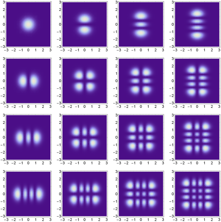
One set of solutions to the paraxial wave equation are Gauss-Hermite beams, which have an intensity profiles like those shown in Figure 2. These are the same solutions as for the quantum simple harmonic oscillator, a topic that could be further explored as a final project.
The simplest of these solutions is the Gaussian beam, which has an electric field given by
\[\vec{E}(x,y,z,t) = \vec{E}_0\frac{w_0}{w(z)}exp\left(-\frac{x^2+y^2}{w^2(z)}\right)exp\left(ik\frac{x^2+y^2}{2R(z)}\right)e^{-i\zeta(z)}e^{i(kz-\omega t)}\text{,}\quad\quad\](8)
where \(\vec{E_0}\) is a time-independent vector (orthogonal to propagation direction \(\hat{z}\)) whose magnitude denotes the amplitude of the laser’s electric field and the direction denotes the direction of polarization. The beam radius \(w(z)\) is given by
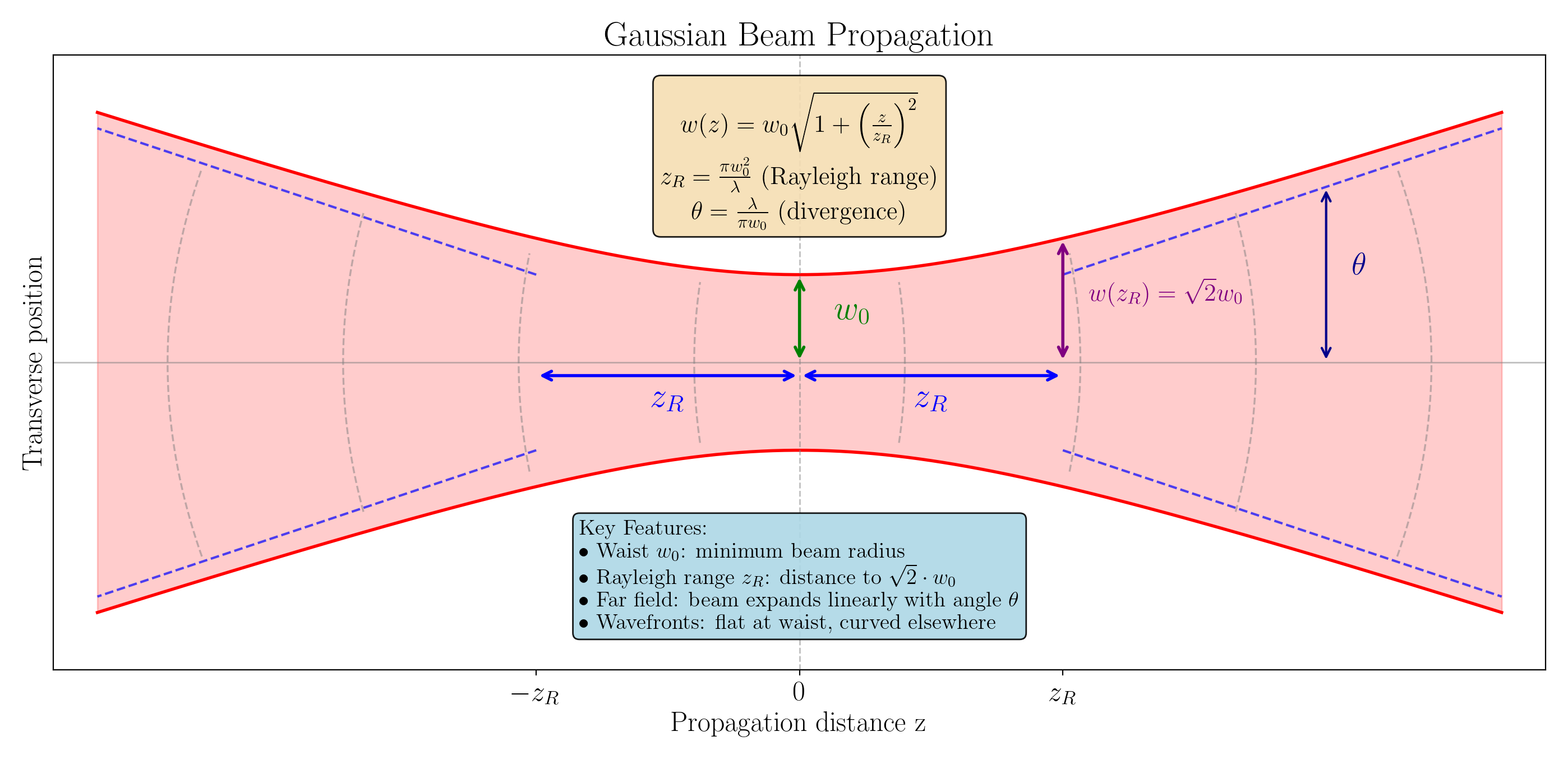
\[w(z)=w_0\sqrt{1+\left(\frac{\lambda z}{\pi w_0^2}\right)^2}\text{.}\](9)
Terminology note: The parameter \(w\) is called the beam radius—the distance from the beam axis to where the intensity falls to \(1/e^2\) of its peak value. This follows from the Gaussian intensity profile \(I \propto e^{-2r^2/w^2}\): at \(r = w\), the intensity is \(e^{-2} = 1/e^2\) of the maximum. You’ll explore this connection further below. The beam diameter would be \(2w\). Some texts use “beam width” for \(w\), but we use “beam radius” consistently in this lab to avoid confusion with the everyday meaning of “width” as a full extent.
\(R(z)\), the radius of curvature of the wavefront, is given by
\[R(z)=z\left(1+\left(\frac{\pi w_0^2}{\lambda z}\right)^2\right)\text{,}\](10)
and the Gouy phase is given by
\[\zeta(z)=\arctan\frac{\lambda z}{\pi w_0^2}\text{.}\](11)
The remarkable thing about all these equations is that only two parameters need to be specified to give the whole beam profile: the wavelength \(\lambda\) and the beam waist \(w_0\), which is the narrowest point in the beam profile.
There is a more general set of Hermite Gaussian modes which are shown in Figure 2. The laser cavity typically produces the (0,0) mode shown in the upper left corner, but an optical cavity can also be used to create these other modes – a topic that can be explored in the final projects.
5.3 Physical Intuition Check
Before applying these equations, test your physical understanding. Answer each question without looking at the equations, then verify with a calculation.
Scaling the waist: If you double the beam waist \(w_0\), what happens to:
- The divergence angle \(\theta = \lambda / (\pi w_0)\) in the far field?
- The Rayleigh range \(z_R = \pi w_0^2 / \lambda\)?
Intuition check: A wider waist means the beam is more collimated (less divergent). Does your answer reflect this?
Distance to double: At what distance from the waist does the beam radius double (i.e., \(w(z) = 2w_0\))?
Hint: Set up the equation and solve for \(z\) in terms of \(z_R\). The answer is a simple multiple of the Rayleigh range.
Wavelength dependence: Two lasers have identical beam waists \(w_0\), but one is red (633 nm) and one is blue (450 nm). Which beam diverges more rapidly? Why?
Conservation of energy: As the beam expands, the width increases but the total power stays constant. What must happen to the peak intensity \(I_{max}\) as \(z\) increases? Write a proportionality relationship.
Beam quality check: You measure a beam radius of \(w = 0.8\) mm at \(z = 1\) m from the laser. Assuming \(\lambda = 633\) nm, what is the minimum possible beam waist? (Hint: The waist could be inside or outside the laser cavity.)
Record your answers in your notebook. Getting physical intuition wrong is valuable—it reveals gaps in understanding that equations alone can hide.
5.4 Trying out the Gaussian beam model
In the first week of the lab, we assumed the intensity profile of the Gaussian beam was given by \(I(x,y)=I_{max}e^{-2(x^2+y^2)/w^2}\). The equation for the electric field of the Gaussian Beam in Equation 8 looks substantially more complicated.
- How are the expressions for electric field and intensity related?
- Is Equation 8 consistent with the simple expression for intensity \(I(x,y)=I_{max}e^{-2(x^2+y^2)/w^2}\)?
The Gaussian beam equations given in Equations 8 -11 assume the beam comes to its narrowest width (called the beam waist, \(w_0\)) at \(z=0\).
- How would you rewrite these four equations assuming the beam waist occurs at a different position \(z=z_w\)?
- One way to check your answer is to make sure the equations simplify to Equations 8 -11 in the special case of \(z_w=0\).
You will fit actual beam radius data in lab today using these modified equations.
5.5 Beyond Beam Radius: The Unmeasured Parameters
The Gaussian beam solution contains three key z-dependent quantities: the beam radius \(w(z)\), the wavefront radius of curvature \(R(z)\), and the Gouy phase \(\zeta(z)\). In Week 4, you will measure only \(w(z)\) using the knife-edge technique. What about the others?
5.5.1 What we can and cannot measure with a knife edge
The knife-edge profiler measures intensity as a function of position. This directly gives you \(w(z)\), the beam radius. However:
\(R(z)\) (radius of curvature): This describes how the wavefronts are curved. Larger \(R\) means flatter (less curved); \(R = \infty\) is perfectly flat. The wavefronts are flattest at the waist, most curved at \(z = z_R\), then become flatter again far away. A knife edge only sees intensity, not phase, so it cannot measure \(R(z)\) directly.
\(\zeta(z)\) (Gouy phase): This is a phase shift that accumulates as the beam passes through its waist. Like \(R(z)\), it requires phase-sensitive measurements.
5.5.2 How would you measure \(R(z)\)?
If you wanted to measure the wavefront curvature, you would need interferometry—combining your beam with a reference beam and analyzing the interference pattern. The spacing and curvature of interference fringes reveals \(R(z)\).
Think about it: Near the waist, \(R(z) \to \infty\) (flat wavefronts). At \(z = z_R\), \(R\) reaches its minimum value of \(2z_R\) (maximum curvature). Far from the waist, \(R(z) \approx z\)—the wavefronts are spherical surfaces centered on the waist, but with large radius (gentle curvature). This non-monotonic behavior means the wavefronts curve most strongly at one Rayleigh range from the waist, not at large distances.
5.5.3 How would you measure \(\zeta(z)\)?
The Gouy phase shift is subtle—it’s a \(\pi\) total phase change as the beam goes from \(z = -\infty\) to \(z = +\infty\) through the waist. Detecting it requires:
- Interferometry with a reference beam that bypasses the focus
- Mode-matching experiments where the Gouy phase affects coupling efficiency
The Gouy phase has practical consequences: it affects the resonant frequencies of laser cavities and the focal properties of lens systems.
5.5.4 Why does the beam radius \(w(z)\) suffice for this lab?
For characterizing a laser beam’s propagation, \(w(z)\) is often the most practically important parameter because:
- It determines the spot size for any application (machining, microscopy, communications)
- Combined with the wavelength \(\lambda\), measurements of \(w(z)\) at multiple positions uniquely determine the waist \(w_0\) and waist position \(z_w\)
- Once you know \(w_0\), you can calculate \(R(z)\) and \(\zeta(z)\) from the equations—you don’t need to measure them separately
Reflection: In what applications might you actually need to measure \(R(z)\) or \(\zeta(z)\) rather than just calculating them from \(w_0\)? (Hint: The theoretical equations assume a perfect Gaussian beam. Consider what happens with aberrated optics, higher-order modes, or beams of unknown origin.)
6 Setting Up the Motor Controller
You will use Python to automate beam profile measurements by controlling a motorized translation stage. This section guides you through setting up and verifying the motor controller hardware this week, so you’re ready for systematic data collection in Week 4.
If you did not complete section 10 from week 1 (manual data collection), you must do that now before proceeding as you will need to remove the micrometer installed in the translation stage in the next section.
6.1 Hardware Overview
The Thorlabs KST101 and ZST225B is a stepper motor controller and stepper motor actuator that can precisely position a translation stage. You will use it to move a razor blade across the laser beam while the DAQ records the photodetector signal.
For detailed specifications and documentation, see the KST101 controller and ZST225B actuator product pages on the Thorlabs website.
The physical connections are:
- Motor Controller (KST101):
- Install the ZST225B actuator into the translation stage (removing the manual micrometer that was used in week 1)
- Connect the ZST225B actuator to the KST101 controller
- Connect the power supply to the KST101
- Do not connect USB yet — you must first configure the stage type (see “Verifying the Motor Connection” below)
- Optical Setup (for testing):
- Position the photodetector after the knife-edge in the beam path
- Ensure the beam passes cleanly through when the razor is fully retracted
6.2 Software Prerequisites
This section is for users who want to install the software on their personal devices. The lab laptops already have this installed.
6.2.1 1. Thorlabs Kinesis SDK
Download and install from the Thorlabs website: https://www.thorlabs.com/software_pages/ViewSoftwarePage.cfm?Code=Motion_Control
Important: Choose the correct version:
- If you have 32-bit Python: Install the 32-bit Kinesis software
- If you have 64-bit Python: Install the 64-bit Kinesis software
To check your Python version, run:
import sys
print(sys.maxsize > 2**32)  # True = 64-bit, False = 32-bit
6.2.2 2. Python Packages
Install the required packages:
pip install pythonnet uncertaintiespythonnet: Required for interfacing with Thorlabs Kinesis motor controluncertainties: Required for error propagation calculations in the analysis section
(You should already have nidaqmx,
numpy, scipy, and
matplotlib from Week 2.)
6.3 Verifying the Motor Connection
6.3.1 Test that Windows Recognizes the Device
Important: Before using Python, the KST101 must be configured with the correct stage type. This is a one-time setup stored in the controller’s memory.
- Without connecting the USB cable from the KST101 to your PC, power on the KST101
- Press the Menu button
- Use the wheel to navigate to “10 Select Stage”
- Press the Menu button again
- Select your actuator type (ZST225) by using the wheel to navigate
- Press the Menu button again to save and exit
- Power cycle the controller using the power switch on the KST101 (unplugging it will not save the settings)
- After power cycling, plug the USB cable from the KST101 into your PC
- Open the Kinesis app
- Connect to the KST101 from the Kinesis app if it’s not connected automatically
- Verify that the section in the bottom right corner of the
KCube Stepper Motor Controllerwindow indicatesActuator: HS ZST225B- if it’s listed as another type, click on this section to change it - Close the Kinesis app
After completing these steps, you should not need to do this again as long as you continue to use the same laptop and KST101.
6.3.2 Test Basic Motor Communication
Run this test script to verify Python can communicate with the motor:
import clr
import sys
import time

# Add Kinesis .NET assemblies
sys.path.append(r"C:\Program Files\Thorlabs\Kinesis")
clr.AddReference("Thorlabs.MotionControl.DeviceManagerCLI")
clr.AddReference("Thorlabs.MotionControl.KCube.StepperMotorCLI")

from Thorlabs.MotionControl.DeviceManagerCLI import DeviceManagerCLI
from Thorlabs.MotionControl.KCube.StepperMotorCLI import KCubeStepper

# Build device list
DeviceManagerCLI.BuildDeviceList()

# Get list of connected devices
device_list = DeviceManagerCLI.GetDeviceList()
print(f"Found {len(device_list)} device(s):")
for serial in device_list:
    print(f"  Serial: {serial}")
If this shows your device serial number, the connection is working.
6.3.3 Test Motor Movement
Caution: Make sure the translation stage has room to move before running this test. Check that nothing is blocking the stage mechanically.
Note: This test uses relative movement, so you don’t need to home first. However, you should home the stage (see next section) before taking actual measurements.
import clr
import sys
import time

sys.path.append(r"C:\Program Files\Thorlabs\Kinesis")
clr.AddReference("Thorlabs.MotionControl.DeviceManagerCLI")
clr.AddReference("Thorlabs.MotionControl.KCube.StepperMotorCLI")
clr.AddReference("Thorlabs.MotionControl.GenericMotorCLI")

from Thorlabs.MotionControl.DeviceManagerCLI import DeviceManagerCLI
from Thorlabs.MotionControl.KCube.StepperMotorCLI import KCubeStepper
from System import Decimal

# Replace with your serial number
SERIAL_NUMBER = "26004813"  # Check the display on your KST101

DeviceManagerCLI.BuildDeviceList()
device = KCubeStepper.CreateKCubeStepper(SERIAL_NUMBER)

try:
    device.Connect(SERIAL_NUMBER)
    print("Connected!")

    # Wait for settings to initialize
    device.WaitForSettingsInitialized(5000)
    device.StartPolling(50)
    time.sleep(0.5)
    device.EnableDevice()
    time.sleep(0.5)

    # Load motor configuration
    config = device.LoadMotorConfiguration(SERIAL_NUMBER)

    # Get current position
    pos = device.Position
    print(f"Current position: {pos} mm")

    # Move relative (small test movement)
    print("Moving 0.5 mm...")
    device.SetMoveRelativeDistance(Decimal(0.5))
    device.MoveRelative(60000)  # 60 second timeout

    new_pos = device.Position
    print(f"New position: {new_pos} mm")

finally:
    device.StopPolling()
    device.Disconnect()
    print("Disconnected")
After you’ve successfully run the code above, verify that the position value reported from Python matches the position that is indicated on the screen of the KST101 - if these numbers disagree, please let your instructor or the technical staff know before proceeding.
6.3.4 Homing the Stage
When the motor controller is powered on, it doesn’t know the stage’s absolute position. Homing moves the stage to a known reference point (typically one end of travel), establishing a reliable zero position.
When to home:
- Once at the start of each measurement session
- After the stage hits a travel limit
- If the reported position seems incorrect
To home the stage in Python:
# After device.EnableDevice() and loading configuration:
print("Homing...")
device.Home(60000)  # 60 second timeout
print(f"Homed. Position: {device.Position} mm")
The stage will move to its home position (near 0 mm). This may take several seconds. You can also home the stage using the front panel: press the Menu button and use the wheel to navigate to the Home option.
6.4 Motor Controller Troubleshooting
“Device not found” Error:
- Check USB connection
- Verify serial number matches the display on the KST101
- Make sure no other software (APT User, Kinesis) is using the motor
Motor Doesn’t Move:
- Ensure power is connected to the KST101
- Check that the stage isn’t at a travel limit
- Verify the stage type is configured correctly in Kinesis (ZST225B)
Python Import Errors:
- Ensure Kinesis SDK is installed and matches Python architecture (32/64-bit)
- Check that the path to Kinesis DLLs is correct
6.5 Exercise: Verify Your Setup
Before leaving lab today, verify that:
- The DAQ can read voltages from the photodetector
- Python can connect to the motor controller
- The motor moves when commanded
- The stage has been homed successfully
- You have noted your motor’s serial number: ____________
This setup will be essential for the automated measurements in Week 4.
Note on AI assistance: The motor control code involves interfacing with hardware libraries that have specific requirements (correct DLL paths, serial numbers, initialization sequences). You may use AI to help generate this boilerplate code. What matters is that you can (1) verify the hardware is responding correctly, (2) diagnose common connection failures, and (3) modify parameters like movement distance and velocity. The Troubleshooting Reflection below tests these skills.
6.6 Troubleshooting Reflection
Developing systematic troubleshooting skills is essential for experimental physics. Answer this question in your notebook:
If the motor doesn’t respond to Python commands, what troubleshooting steps would you take?
List at least three things you would check, in order of likelihood, and explain your reasoning. Consider:
- What are the most common failure modes?
- What’s the quickest way to isolate hardware vs. software issues?
- How would you determine if the problem is with Python, the USB connection, or the motor itself?
This systematic approach to troubleshooting will serve you well in Week 4 and beyond.
7 Taking Your First Automated Beam Profile
Now that you have the motor controller working, take a complete beam profile measurement. Think of this as a trial run—you’re getting the kinks out before Week 4’s systematic data collection. This serves two purposes: (1) verify your entire measurement system works end-to-end, and (2) generate real data for the error propagation analysis later in this lab session.
Before you start, make a prediction: Will your automated data be more or less noisy than your manual measurements from Week 1? Why? Record your prediction in your notebook—you’ll revisit this after taking data.
7.1 Measurement Procedure
Here is an overview of the measurement process. The sections that follow provide details on integrating your code and checking your data quality.
Position the knife-edge assembly at a known distance from the laser (measure and record this distance—you’ll need it for analysis).
Set up the measurement:
- Ensure the photodetector is receiving the full beam when the knife-edge is retracted
- Use the gain setting you determined in Week 2
- Verify DAQ is reading reasonable voltages
Choose your measurement parameters:
Think about what step size will give you good data:
- Recall your beam radius \(w\) from your Week 1 manual measurement
- The transition region where voltage changes spans roughly \(2w\)
- You want at least 10-15 points in the transition region to constrain your fit
- What step size does this imply?
In Week 4, you will revisit this choice more systematically based on your specific beam radius and measurement goals.
Take the beam profile:
- Move the knife-edge across the beam using your chosen step size
- At each position, record the motor position and photodetector voltage
- Continue until the beam is fully blocked (voltage reaches dark level)
Save your data with a descriptive filename including the date and z-position (e.g.,
beam_profile_2026-01-27_z50cm.csv). In Week 4, you’ll collect profiles at multiple z-positions, so systematic naming will help you keep track of which data came from where.
7.2 Integrating Motor and DAQ
To automate beam profiling, you need to combine motor positioning with voltage reading. The code below shows the DAQ portion, but the motor movement is commented out.
To complete this code, you need a
move_to() function. You have two
options:
Adapt the relative movement code from the verification section above (hint: use
device.MoveTo(Decimal(position_mm), timeout_ms)for absolute positioning)Reference the complete motor control documentation at Thorlabs Motor Control with Python, which includes a working
move_to()function and a completerun_position_scan()example.
Some decisions you’ll need to make: How long should you wait for vibrations to settle after each move? What position range covers the full transition from unblocked to fully blocked? How many samples should you average at each position to reduce noise?
import time
import numpy as np
import nidaqmx

# Configuration
positions = np.arange(0, 3, 0.1)  # 0 to 3 mm in 0.1 mm steps
data = []

for pos in positions:
    # Move motor to position (use your motor control code)
    # device.MoveTo(Decimal(pos), 60000)
    time.sleep(0.3)  # Wait for motor to settle

    # Read voltage (change "Dev1/ai0" to match your DAQ channel if needed)
    with nidaqmx.Task() as task:
        task.ai_channels.add_ai_voltage_chan("Dev1/ai0")
        voltage = np.mean(task.read(number_of_samples_per_channel=100))

    data.append([pos, voltage])
    print(f"Position: {pos:.2f} mm, Voltage: {voltage:.4f} V")

# Save data
np.savetxt('beam_profile_week3.csv', data, delimiter=',',
           header='Position (mm), Voltage (V)', comments='')
7.3 Quick Check
Before proceeding to the analysis section (where you’ll fit this data to extract beam radius \(w\)), verify your data looks reasonable:
- Does the voltage transition smoothly from high to low? (Some scatter is normal, but the trend should be clear.)
- Does your data span the full range from maximum voltage (beam unblocked) to minimum voltage (beam fully blocked)?
- Do you have at least 10 points in the transition region where the voltage is changing?
If the transition is unclear or you have too few points, retake the measurement with smaller step sizes or a different position range.
Revisit your prediction: Was your automated data more or less noisy than your Week 1 manual data? What might explain the difference?
8 Applying Theory to Your Measurements
This section connects the Gaussian beam theory from your prelab to your actual measurements. You’ll learn error propagation by applying it to your own data—not abstract examples.
8.1 Error Propagation: From Measured to Derived Quantities
The quantity of interest in an experiment is often derived from other measured quantities. For example, you’ll derive beam radius \(w\) from your knife-edge data, then use \(w\) at multiple positions to determine the beam waist \(w_0\).
8.1.1 The General Equation
Suppose you want to derive a quantity \(z\) from measured quantities \(a, b, c, ...\). The mathematical function is \(z = z(a, b, c, ...)\). The propagated uncertainty in \(z\) is:
\[\sigma_z^2 = \left( \frac{\partial z}{\partial a}\right)^2\sigma_a^2+\left( \frac{\partial z}{\partial b}\right)^2\sigma_b^2+\left( \frac{\partial z}{\partial c}\right)^2\sigma_c^2+ \ ...\text{.}\]
This comes directly from calculus—it’s the linear approximation of how fluctuations in inputs cause fluctuations in outputs.
8.1.2 Error Propagation in Python
For complex calculations, the uncertainties
package automatically tracks error propagation:
from uncertainties import ufloat
from uncertainties.umath import sqrt

# Define values with uncertainties
V = ufloat(5.0, 0.1)   # 5.0 ± 0.1 V
I = ufloat(0.5, 0.02)  # 0.5 ± 0.02 A

# Calculate - uncertainty propagates automatically
R = V / I
print(f"R = {R}")  # Shows value ± uncertainty
8.2 Fitting Your Beam Profile Data
Now fit your beam profile data to extract the beam radius.
8.2.1 Step 1: Load and Plot Your Data
import numpy as np
import matplotlib.pyplot as plt
from scipy.optimize import curve_fit
from scipy.special import erf

# Load your data
data = np.loadtxt('beam_profile_week3.csv', delimiter=',', skiprows=1)
position = data[:, 0]  # mm
voltage = data[:, 1]   # V

# Plot raw data
plt.figure(figsize=(10, 6))
plt.plot(position, voltage, 'bo', label='Data')
plt.xlabel('Position (mm)')
plt.ylabel('Voltage (V)')
plt.title('Beam Profile - Week 3')
plt.grid(True, alpha=0.3)
plt.show()
8.2.2 Step 2: Define and Fit the Error Function Model
The knife-edge measurement gives an integrated Gaussian, which is the error function:
\[V(x) = \frac{V_{max} - V_{min}}{2} \left[1 - \text{erf}\left(\frac{\sqrt{2}(x - x_0)}{w}\right)\right] + V_{min}\]
def beam_profile(x, V_max, V_min, center, width):
    """Error function model for knife-edge beam profile.

    Parameters:
        x: position (mm)
        V_max: maximum voltage when beam is unblocked (V)
        V_min: minimum voltage when beam is blocked (V)
        center: beam center position (mm)
        width: beam radius w (mm)

    Note: This form uses V_max/V_min instead of amplitude/offset
    for physical clarity. The forms are equivalent:
        amplitude = (V_max - V_min) / 2
        offset = (V_max + V_min) / 2
    """
    return (V_max - V_min) / 2 * (1 - erf(np.sqrt(2) * (x - center) / width)) + V_min

# Initial guesses
V_max_guess = np.max(voltage)
V_min_guess = np.min(voltage)
center_guess = position[len(position)//2]
width_guess = 0.5  # mm

p0 = [V_max_guess, V_min_guess, center_guess, width_guess]

# Fit the data (bounds ensure width stays positive)
bounds = ([0, 0, -np.inf, 0], [np.inf, np.inf, np.inf, np.inf])
popt, pcov = curve_fit(beam_profile, position, voltage, p0=p0, bounds=bounds)
perr = np.sqrt(np.diag(pcov))

# Extract results
V_max, V_min, center, width = popt
V_max_err, V_min_err, center_err, width_err = perr

print(f"Beam radius: w = {width:.4f} ± {width_err:.4f} mm")
print(f"Beam center: x0 = {center:.4f} ± {center_err:.4f} mm")
Troubleshooting fit issues:
- Fit doesn’t converge: Check that your
initial guesses are reasonable. Try adjusting
width_guessbased on your data’s transition region. - Very large uncertainties: You may not have enough points in the transition region. Retake data with smaller step sizes.
- Fit looks wrong: Plot your data first and verify it shows a clear S-curve transition. If the curve is inverted, check the sign in the error function model.
8.2.3 Step 3: Plot the Fit
# Generate smooth curve for plotting
x_fit = np.linspace(position.min(), position.max(), 200)
v_fit = beam_profile(x_fit, *popt)

plt.figure(figsize=(10, 6))
plt.plot(position, voltage, 'bo', label='Data')
plt.plot(x_fit, v_fit, 'r-', label=f'Fit: w = {width:.3f} ± {width_err:.3f} mm')
plt.xlabel('Position (mm)')
plt.ylabel('Voltage (V)')
plt.title('Beam Profile with Error Function Fit')
plt.legend()
plt.grid(True, alpha=0.3)
plt.savefig('beam_profile_fit.png', dpi=150)
plt.show()
Record in your notebook:
- Beam radius: $w = $ _______ \(\pm\) _______ mm
- Measurement position: $z = $ _______ m from laser
Connection to Week 2: The uncertainty in your fit parameters depends on the noise level in your voltage measurements. Your Week 2 noise characterization tells you what σ_V to expect at your gain setting. Look at the residuals (data minus fit)—does their scatter match your predicted noise level? If the residuals are much larger than expected, you may have additional noise sources (vibration, beam drift) affecting your measurement.
8.3 Predicting Week 4 Results
Now use your measured beam radius to make predictions for Week 4. This is where error propagation becomes practical.
8.3.1 Step 1: Estimate Beam Waist from Your Measurement
Using the Gaussian beam equation:
\[w(z) = w_0\sqrt{1+\left(\frac{\lambda (z - z_w)}{\pi w_0^2}\right)^2}\]
If we assume \(z_w \approx 0\) (beam waist at laser output), we can estimate \(w_0\) from a single measurement. Rearranging:
from uncertainties import ufloat
from uncertainties.umath import sqrt
import numpy as np

# Your measured values (replace with your actual data)
w_measured = ufloat(0.52, 0.03)  # mm - USE YOUR VALUE
z_measured = ufloat(1.5, 0.01)   # m - USE YOUR VALUE
wavelength = 632.8e-9  # m (He-Ne laser)

# Convert w to meters
w_m = w_measured * 1e-3

# For a beam at distance z from waist, we can estimate w0
# This is approximate - assumes z >> z_R (far from waist)
# w ≈ w0 * z * λ / (π * w0²) = z * λ / (π * w0)
# So w0 ≈ z * λ / (π * w)
w0_approx = z_measured * wavelength / (np.pi * w_m)

print(f"Approximate beam waist: w0 ≈ {w0_approx*1e6:.1f} μm")

# Check if far-field approximation is valid (z >> z_R)
z_R_approx = np.pi * w0_approx**2 / wavelength
print(f"Estimated Rayleigh range: z_R ≈ {z_R_approx:.2f} m")
print(f"z / z_R = {z_measured.n / z_R_approx.n:.1f} (should be >> 1 for far-field)")
Note: If z/z_R is close to 1, you are not in the far field and this approximation may be inaccurate. This is expected—Week 4’s multi-position measurements and proper fitting will give a more reliable estimate of \(w_0\).
8.3.2 Step 2: Predict Beam Radii at Other Positions
Use error propagation to predict what you’ll measure in Week 4:
# Predict beam radius at different positions
positions = [0.5, 1.0, 1.5, 2.0]  # meters

print("\nPredicted beam radii for Week 4:")
print("-" * 40)
for z in positions:
    z_val = ufloat(z, 0.01)
    z_R = np.pi * w0_approx**2 / wavelength
    w_pred = w0_approx * sqrt(1 + (z_val / z_R)**2)
    print(f"z = {z:.1f} m:  w = {w_pred*1e3:.3f} mm")
8.3.3 Step 3: Record Your Predictions
Fill in this table in your notebook:
| Position \(z\) | Predicted \(w(z)\) | Predicted uncertainty |
|---|---|---|
| 0.5 m | _______ mm | ± _______ mm |
| 1.0 m | _______ mm | ± _______ mm |
| 1.5 m | _______ mm | ± _______ mm |
| 2.0 m | _______ mm | ± _______ mm |
Prediction reflection: If your Week 4 measurements differ significantly from these predictions, what are the most likely causes? List at least two possibilities, and for each one, describe what signature in your Week 4 data would distinguish that cause from the others. (For example: Would the discrepancy be systematic across all positions? Would it affect near-field and far-field measurements differently?)
8.4 Comparing Manual vs. Motor-Controlled Measurements
If you took beam radius measurements manually in Week 1, compare them to today’s motor-controlled measurement:
| Method | Beam radius | Uncertainty | Notes |
|---|---|---|---|
| Week 1 (manual) | _______ mm | ± _______ mm | |
| Week 3 (motor) | _______ mm | ± _______ mm |
Are they consistent within uncertainties? If not, what might explain the difference?
9 Deliverables and Assessment
Your lab notebook should include the following for this week:
9.1 Prelab (complete before lab, ~75 min)
- Paraxial wave equation derivation: show the key steps from Maxwell’s equations to Equation 7
- Physical Intuition Check: answers to all 5 questions
- Gaussian beam model questions: answers to questions 1-4 in “Trying out the Gaussian beam model”
- Beyond Beam Radius reflection: when might you need to measure \(R(z)\) or \(\zeta(z)\) directly?
9.2 In-Lab Documentation
9.2.1 Phase 2: Measurement (~60 min)
- Motor controller verification:
- Completed setup checklist (DAQ, motor connection, movement test)
- Motor serial number recorded
- Troubleshooting reflection
- Beam profile data:
- Raw data file saved
- Position of measurement from laser: $z = $ _______ m
- Quick check: does data show clean transition?
9.2.2 Phase 3: Analysis (~60 min)
- Beam profile fit:
- Fit plot showing data and error function model
- Extracted beam radius: $w = $ _______ \(\pm\) _______ mm
- Error propagation and predictions:
- Estimated beam waist \(w_0\)
- Predicted beam radii at 4 positions for Week 4
- Prediction reflection (what could cause disagreement?)
- Comparison (if Week 1 data available):
- Manual vs. motor-controlled beam radius comparison
9.3 Code Deliverables
- Motor communication test script
- Beam profile fitting script
9.4 Reflection Questions
What was the dominant source of uncertainty in your beam radius measurement? How could you reduce it?
Based on your motor controller setup experience, what was the most challenging part? How would you help a classmate who encountered the same issue?
Look at your predicted beam radii for Week 4. Which measurement position will have the largest relative uncertainty (σ_w / w)? Why?