PHYS 4430

Gaussian Beams - Week 1

1 Goals

In the first week of the guided Gaussian Beams lab, you learn about mounting optics and photodetectors and try out some techniques that are generally useful in optics labs and elsewhere. In particular, you will set up a simple optics system for measuring the width of a laser beam and in the process will have to mount and align the laser and optics.

2 Lab Notebook

Your lab notebook will play an important role in this course. You will use your notebook for keeping records of many things including:

Answering prelab questions from the lab guides
Answering in-lab question from the lab guides
Recording data
Including plots of data
Analysis and results
Diagrams and pictures
Procedures of experiments that you design

The lab notebook will be an important part of your grade because learning to keep a good lab notebook is an important part of your professional development.

3 Definitions

Optic – Any optical component that manipulates the light in some way. Examples include lenses, mirrors, polarizing filters, beam splitters, etc.

Optomechanics – This category includes optics mounts and the components to align them. Examples in the lab include post, post holders, bases, lens mounts, adjustable mirror mounts, rotation mounts, and translation stages.

4 Setting up the Laser and Mounting Optics

Your group should find an empty optical breadboard workstation in one of the five color coded optics bays in G-214. Spend some time to explore the space and familiarize yourself with the components. The shelf above the breadboard should have:

An oscilloscope
A waveform generator
Triple output DC Power Supply
Set of ball drivers
Optics caddy to hold optics already mounted on 0.5" posts
Set of 1/4-20 and 8-32 screws, setscrews, washers, and nuts

4.1 Cleaning and handling of optical components

It’s very important that you do not handle optical components (lenses, mirrors, polarizers, wave plates, beam splitters, etc.) with your bare hands. The oils on your skin can damage the optics and degrade the light in your experiment. Always handle these components while using latex/nitrile gloves or finger cots, which can be found on the top of the tool cabinets in your optics bay, or on top of the black drawer cabinets in the main lab. This technical note from Newport discusses how to go about cleaning dirty optics, and is also demonstrated in this video. For a more in-depth treatment on cleaning optics, we have a copy of “The Proper Care of Optics: Cleaning, Handling, Storage, and Shipping” by Robert Schalck for reference in the lab (it should be located on top of the black tool cabinets in the main lab).

4.2 Mounting your optomech: bases, post holders, and posts

The two videos linked below provide information and tips on how to use and mount components on the optical breadboards that we have in the lab. Please watch these before proceeding.

Mounting Your Optomech: Bases, Post Holders, and Posts | Thorlabs Insights

Tips for Bolting Post Holders to Optical Tables, Bases, and Breadboards | Thorlabs Insights

Now, we will begin assembling the components.

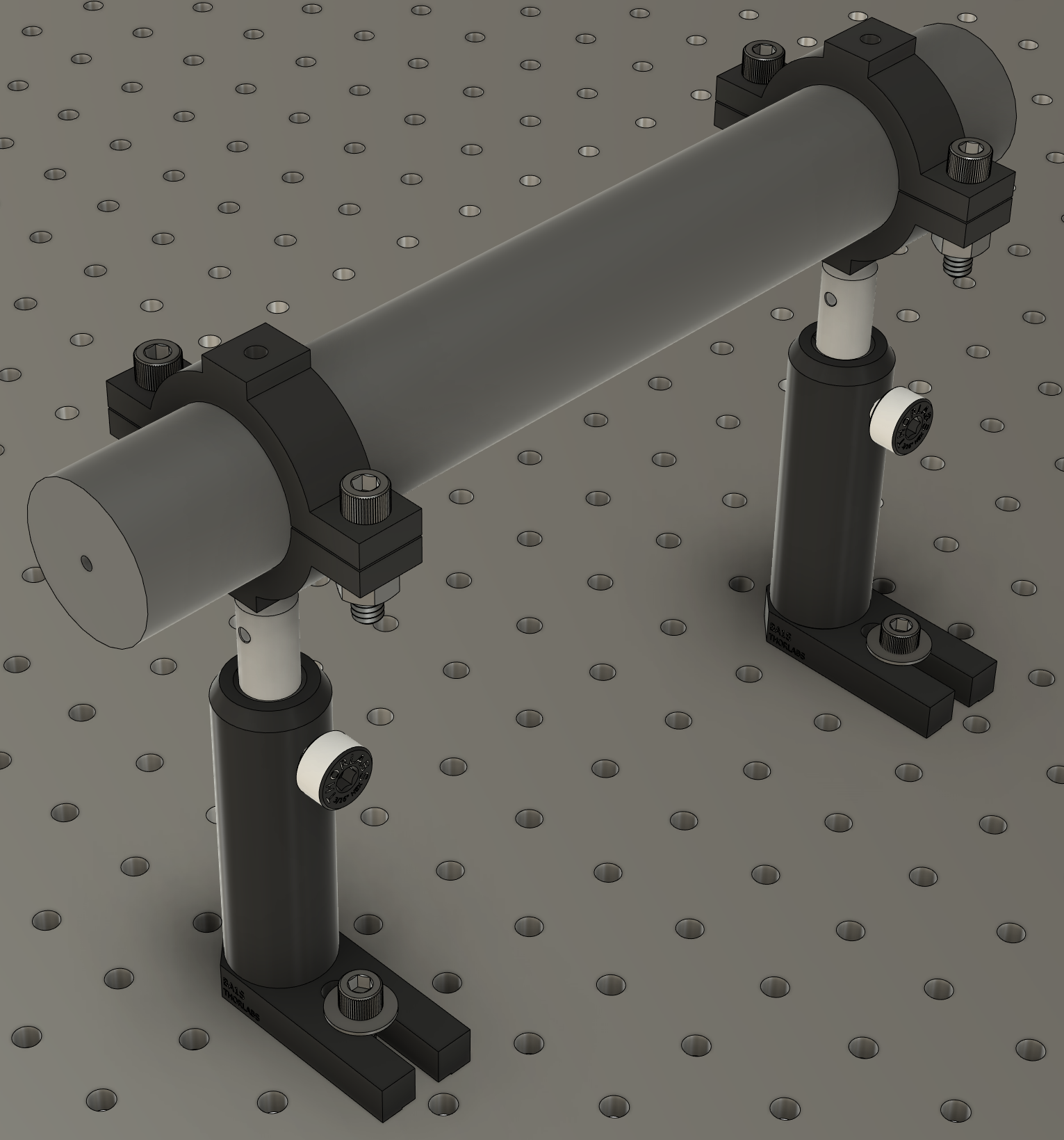
Get a laser and power supply from the “He-Ne Laser” drawer in the colored drawer cabinet found in your chosen or assigned optics bay. You’ll also need two sets of 3D-printed laser tube mounts which you can find in the same drawer (see Figure 1). The bottom mount first gets mounted to an optical post and then the top of the mount can be assembled with ¼-20 socket head cap screw and nut. After both sets of tube mounts are attached to the laser, insert the optical posts into post holders and attach the assembly to the optical table.
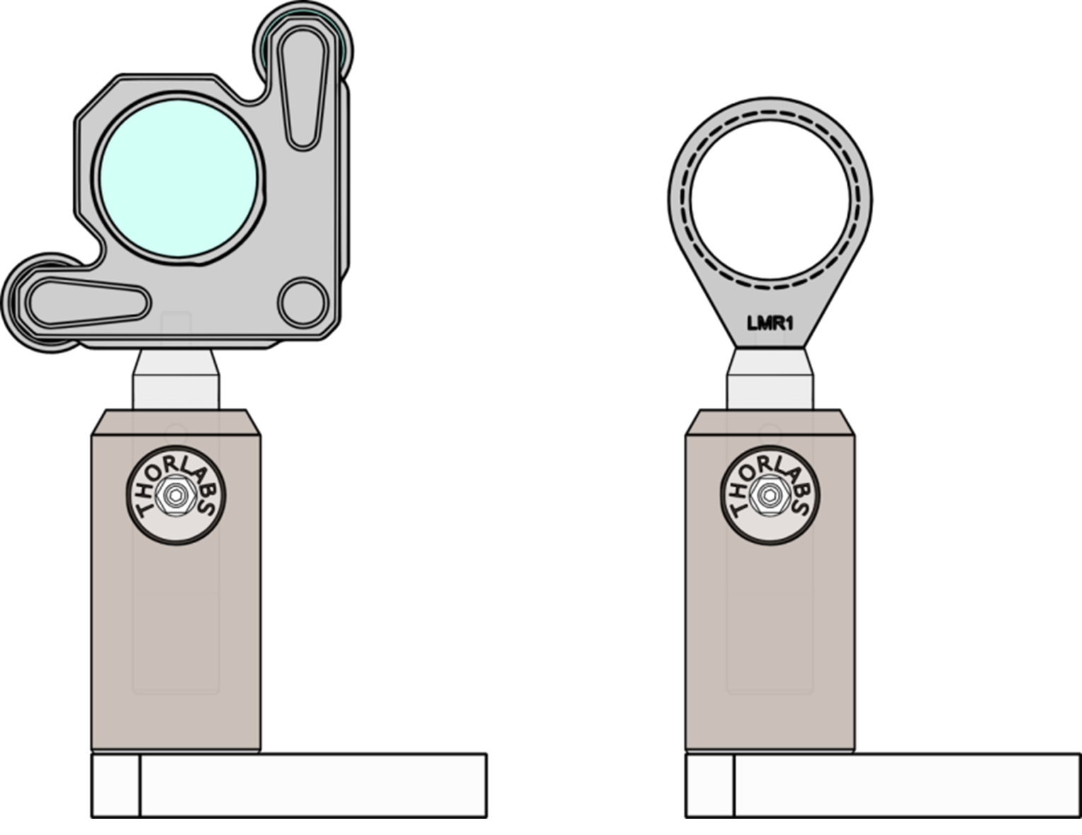
Each person in your group is responsible for assembling a mirror as shown in Figure 2. In the end, you will need at least 2 mirrors to complete the next task. Remember to wear latex/nitrile gloves or finger cots while handling optical components.

As you are mounting the optics, choose the heights so that the laser hits the center of each optic and the beam is parallel to the table.

Figure 1: CAD assembly showing a He-Ne laser mounted to an optical table with the 3D-printed tube mounts that can be found in the tool cabinets in the optical bays of G214.

4.3 Walking a beam

Next, you will align your laser such that beam is aligned parallel to the table. You will do this by using two mirrors and a technique that is called “walking a beam”. This video provides an overview on how to do so. The most relevant information for our lab starts at 4:09 (which the above link should take you to). Also, we have 3D printed beam alignment tools that are used in place of the iris in the video (these can be found in the colored drawer cabinet in your optics bay).

Mount two 3D printed beam alignment discs onto the optical table at the same height above the table.
Use only two mirrors to get the beam to pass through the center of each disc. Having two mirrors allows you to independently adjust the angle and position of your beam.
Draw a diagram in your lab notebook of the configuration of your laser, mirrors, and alignment discs.

Figure 2: Mounting assemblies for a mirror (left) and a lens (right).

5 Modeling Characteristics of the Photodetector

The goal of this part of the lab is to understand a lot about the specifications given on the datasheet for the Thorlabs PDA36A (or PDA36A2) Switchable Gain Amplified Photodetectors (we have both in the lab, so check the model number to know which one you are using). It is important to realize that data sheets (also called spec sheets or specification sheets) provide a model for the realistic behavior of the device. This model can be tested and improved, a process more commonly called “calibration.” Note that there are two power switches, one on the power supply and one on the photodetector. The photodetector will respond to light with the power off but it won’t work well and changing the gain will have little effect.

5.1 Basic function of the amplified photodetector

Spend a few minutes (no more than 10) to write an explanation using words and diagrams to explain the physical mechanism for how the photodetector converts light into voltage. You may use the manufacturer’s specifications sheet (linked to in the section above), trustworthy online resources, a book, etc.
Use the data sheet to estimate the conversion of watts of light into amps of current for Helium-Neon red wavelength (632.8 nm) and for the frequency doubled Nd:YAG laser (Green laser pointer wavelength, 532 nm).
1. How would you convert “amps per watt” into “electrons per photon”?
2. What is the electron/photon conversion efficiency for the red HeNe laser and green doubled Nd:YAG lasers?
3. Is this number less than, equal to, or greater than one? What does this number tell you about how the photodiode works?

5.2 Calibrating the photodetector offset and gain

Calibrating the photodetector is especially important when you take a data set that uses multiple gain settings. Having an accurate calibration of the gain and offset will let you stitch the data together accurately.

Here you will encounter gain values that are presented on a logarithmic $dB$ (decibel) scale, which is obtained by taking $20×log(V_{out}/V_{in})$. For example, $20\ dB$ of gain corresponds to electronic voltage amplification by a factor of 10. A $dB$ scale could also be defined as $10×log(P_{out}/P_{in})$, where $P$ is the power. Explain the conversion between these two scales and why this makes sense.
Calibrating the offset voltage (the output of the photodetector when no light is incident upon the device).
1. Calibrate the offset of the photodetector as a function of gain setting.
2. Quantitatively compare it to the specifications given in the table. Is your measured value within the specified range given on the PDA36A or PDA36A2 photodetector data sheet?
3. What measures did you take to eliminate stray light? Were your measures sufficient for an accurate calibration?
Calibrating the gain.
1. Is it possible to measure the $V/A$ gain for each setting, or can you only measure the change in gain as you switch the settings? Why? Note that this lab only requires relative gain.
2. Make a measurement of the gain or relative gain for most of the gain settings. If you need to adjust the laser power, try blocking part of the beam. Note, you will need to make two measurements at one gain setting when you block the beam. What systematic error sources are of most concern?
3. Quantitatively compare your results with the range of values given on the data sheet. Do you believe your results provide a more accurate estimate of the photodetector gain than the data sheet? Why or why not?
4. Using the appropriate spec sheet and your measurements, what is the power of your laser? Does this agree with the laser power shown on the laser?
5. Hypothetically, how would you measure the absolute gain?

5.3 Follow up

Write mathematical expressions that converts the incident power (the light) $P_{in}$ to the photodetector voltage $V$ and the photodetector voltage $V$ to input power $P_{in}$. Take into account all relevant parameters such as the photodetector gain setting (in $dB$) and offsets.

6 Review of Measurement Uncertainty

When attempting to establish the validity of our experimental results it is always important to quantify the uncertainty. Measurement uncertainty wasn’t invented to make lab classes tedious, rather it is a core part of any experimental work that gives us a way to quantify how much we trust our results.

A simple and rigorous way to make a measurement and estimate its uncertainty is to take $N$ measurements $\{y_1,y_2,\ ...\ ,y_N\}$ and estimate the value by the mean:

\[\overline{y} = \frac{1}{N}{\displaystyle \sum_{i=1}^{N}}y_i\text{.}\]

The estimated uncertainty (standard deviation, $\sigma_y$, or variance, $\sigma_y^2$) of any one measurement is given by

\[\sigma_y^2 = \frac{1}{N-1}{\displaystyle \sum_{i=1}^{N}}(y_i-\overline{y})^2\text{,}\]

while the uncertainty in the mean value $\sigma_{\overline{y}}$ is smaller and is given by

\[\sigma_{\overline{y}}^2 = \frac{\sigma_y^2}{N}\text{.}\]

6.1 Estimating the mean and uncertainty

Make sure that your laser has been turned on for at least 5 minutes so it has had the opportunity to warm up. You will use the photodetector to measure the DC optical power.

6.2 Measurement and uncertainty using the multimeter

Using your digital multimeter, make a table of estimated DC voltages from your photodiode as it is illuminated by your laser and the corresponding uncertainties using the following methods:

“Eyeball” the mean. “Eyeball” the amplitude of the random fluctuations.
Set the multimeter on max/min mode to record the $V_{max}$ and $V_{min}$ fluctuations over a certain time period. You can estimate the mean by $(V_{max}+V_{min})/2$ and the uncertainty by $(V_{max}-V_{min})/2$.
Record the instantaneous voltage reading on the multimeter $N$ times and calculate the estimated uncertainty from the standard deviation.
What is the resolution intrinsic to the multimeter according to the spec sheet (no measurement required)? How does this compare to the observed uncertainty in parts 1-3?

6.3 Measurement and uncertainty using the oscilloscope

Now connect the photodiode to an oscilloscope. Continue the previous table of estimated DC voltages from your photodiode as it is illuminated by your laser and the corresponding uncertainties using the following methods. For each method comment on if and how it depends on the setting for the time scale or voltage scale on the oscilloscope.

“Eyeball” the mean. “Eyeball” the amplitude of the random fluctuations (no cursors or measurement tools).
Use the measurement function on the scope to record the mean and RMS fluctuations.
Use the cursors to measure the mean and size of fluctuations.
Record the voltage from the oscilloscope $N$ times and calculate the estimated uncertainty from the standard deviation.
A comparison with the data sheet is difficult because so many factors affect the observed noise in the oscilloscope. You can find some information here (there is information about the resolution and the DC measurement accuracy) .

6.4 Summary of methods

Make sure to support your answers for each question below.

Did any methods overestimate the uncertainty?
Did any methods underestimate the uncertainty?
How reliable was “eyeballing”?
Did the time scale or voltage scale affect any of the oscilloscope measurements? If yes, how? Does this tell you anything about how to use the scope?
Suppose the light into the photodetector was not constant during the measurements (due to variations of the laser, room lights, etc.). In which estimates of the uncertainty will this be included?
Which method(s) should give a true estimate for the uncertainty?

6.5 Writing numbers and their uncertainty

The convention used in this course is that we:

only display one significant digit of the uncertainty (two are allowed if the first significant digit is a 1).
display the measurement to the same digit as the uncertainty.

The numbers $154\pm 3$, $576.33\pm 0.04$, and $245.1\pm 1.4$ follow theis convention. However, numbers copied from the computer are often displayed as “machine precision” with no regard for significant digits.

Mathematica generated the following fit parameters and corresponding uncertainties:

\[a=-0.6699999999999988 \pm 0.6751049301158053\]

\[b=2.2700000000000005 \pm 0.2035517952102936\]

How should the two Mathematica fit parameters above be rewritten such that they correspond with the convention described above?

7 Measuring the Beam Width

The goal of this section is to develop a measurement technique and analysis scheme to measure the width of a laser beam. The scheme will let you measure the width in one dimension. The technique is most useful for beams that have an approximately Gaussian intensity profile. You will improve and refine this technique in the upcoming weeks of this lab. Note: You may or may not find that completing this section during your lab time this week is challenging due to time constraints. This is okay - get as far as you can now. You’ll have an opportunity to revisit this section during week 3. However, don’t just skip it now as you’ll find the outcomes to be useful in the upcoming weeks.

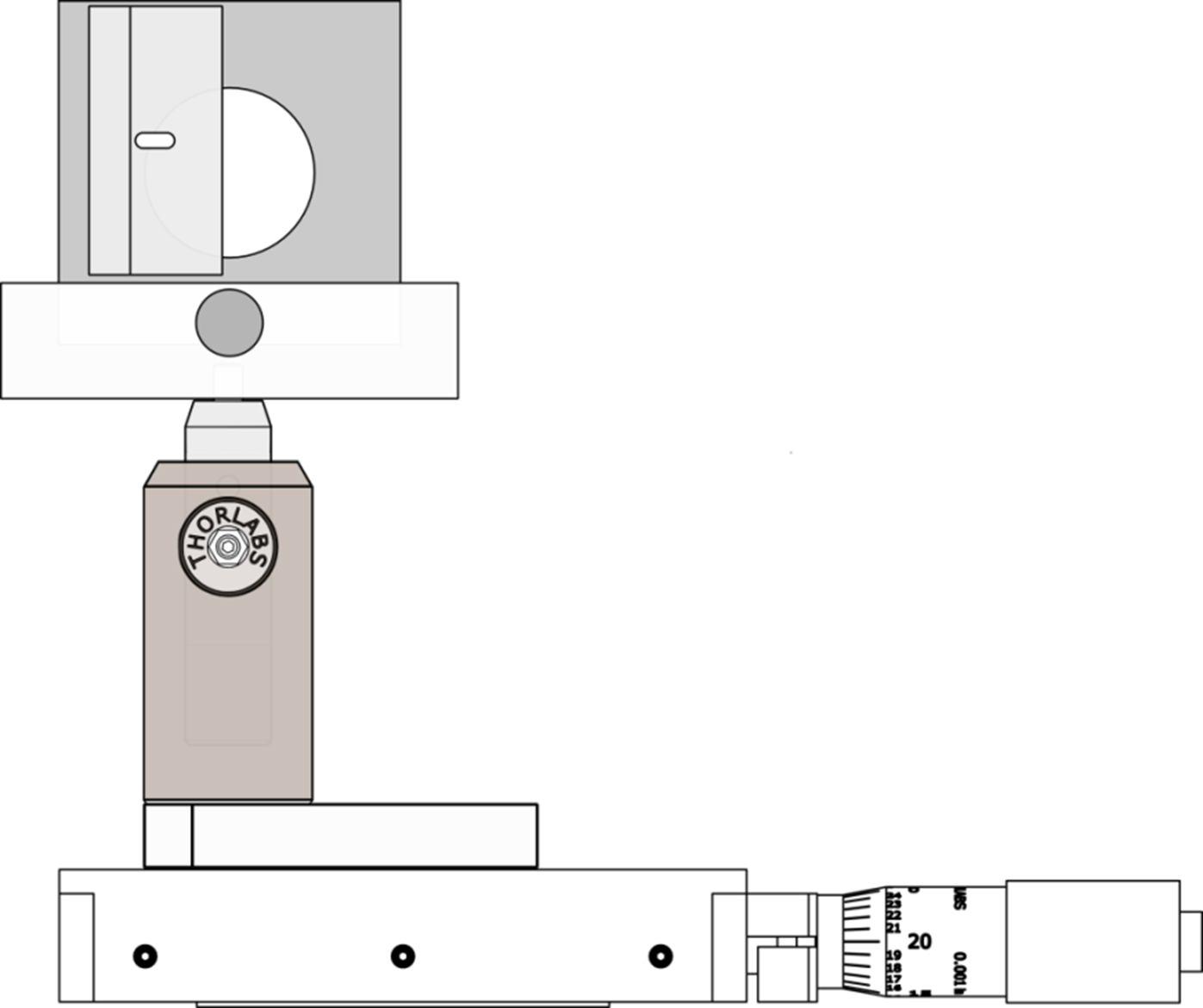
The basic scheme involves measuring the power in the laser beam as the beam is gradually blocked by a knife edge (razor blade) using a setup similar to Figure 3.

Figure 3: Razor blade mounted on a translation stage.

Suppose a laser beam has a Gaussian intensity profile $I(x,y) = I_{max}e^{-2(x^2+y^2)/w^2}$, and is incident upon a photodiode. What is the expression for the power hitting the photodiode when a portion of the beam is blocked by a razor blade?
1. Draw a diagram showing the beam and the razor.
2. Using the above expression for $I(x,y)$, write the mathematical expression for the power incident on the photodiode as a function of razor position. Note, to address this question, you will need to become familiar with the Error Function, $erf(x)$. What assumptions, if any, did you need to make in evaluating the integral? Hint: if you are moving in the $x$ direction, what is going on in the $y$ direction?

7.1 Before you take data: create an analysis function to fit a test set of data

Note: Nonlinear least squares fitting is covered in next week’s prelab. There is also a YouTube video available on least squares fitting in Mathematica.

What is the functional form for your fit function?
Is it a linear or nonlinear fit function? Why?
What are the fit parameters? Why do you need this many?
How do the fit parameters relate to the beam width?
Download this data set.
1. Make a plot of the data.
2. Make a fit and plot it with the data.
3. Check that the fit looks good and you get a beam width of $w=4.52 \times 10^{-4}\ m$. If you get a different value, check with your instructor to understand the problem. What is the uncertainty on your measurement?

7.2 Build your setup for measuring the beam width of your laser

Draw a detailed schematic of the setup (from the laser all the way to the photodetector).
After assembling your experiment, but prior to taking a lot of data, how can you quickly determine if the measurement is working?
Is it preferable to use a digital multimeter or oscilloscope? Why?
Use the measurement scheme to take data of incident power on the photodiode vs. position of the razor. Pay attention to the units of the translation stage. Pick a position where your beam has a measurable width and measure it. Justify your choice.

7.3 Analysis of the random uncertainty sources

What are possible sources of random uncertainty in the photodetector voltage?
How would you estimate the uncertainty in the photodetector voltage measurement?
What is the largest source of uncertainty? Why?

7.4 Analysis of the real data

Use the analysis procedures verified in section 7.1 to find the beam width for your data. Be sure to include the uncertainty.
Plot your fit together with your data to make sure it is good.

8 Postlab

Please choose either Mathematica, Matlab, or Python for this assignment. Both Mathematica and Matlab licenses are provided by CU and Python is free. You must submit both code and results. Note that the following assignment was created based on Mathematica and Matlab.

Evaluate the following math expressions:
1. $e^{1.6\pi j}$
2. $4i\pi+e^{7\pi /4}$
3. $sin^2(\frac{\pi}{5})$
4. $log(3+\sqrt{3})$
5. $|3+4i|^{2/3}$
Plot the following functions at the given ranges. Make sure to add appropriate $x$ and $y$-axis ticks and numeric labels at the ticks locations.
1. Plot $sin^2~\theta$ vs. $\theta$ in the range $0\le\theta\le 6\pi$. Add the legend that indicate the name of the function used.
2. Plot $sin~2t$ and $cos~5t$ together (using different colored lines) on the sample for $t$ in the range of $0\le t \le 10$.
Plot the following data set (wavelength, $\lambda$, and the corresponding index of refraction, $n$, of a particular type of glass):

\[ \lambda~ [{\rm \mu m}]: 0.375, ~ 0.419,~0.558,~ 0.612,~0.744,~0.821 \\ n:1.553,~1.531,~1.521,~1.516,~1.513,~1.511 \]
1. Make a plot of $n$ vs. $\lambda$. Which variable would you choose for $x$-axis? Please make sure to add the axes names and appropriate ticks for each axis.
2. Add lines to connect each points. What can you tell about the relation between the wavelength and the index of refraction from this plot?
3. Provide your code to make your plot from 8.3.1 including the following:
  1. Title of “Refraction index as a function of $\lambda$”.
  2. Add the linear fitting line $ y= ax +b$, where $y$ corresponds to $n$ and $x$ to $\lambda$ on the data.
  3. Include the fitting linear equation on the plot.
4. If you would like to display the $x$-axis only below $0.6\mu m$ (i.e. $\lambda \le 0.6~ \mu m$), how can you do that?
Familiarize yourself with the HELP functions of your chosen software package and perform the following tasks and answer the questions.
1. Make a contour plot of any function of $z=f(y,x)$ of your choice.
2. What are the built-in function names for:
  1. Inverse sine function ($\sin^{-1} x$)
  2. Hyperbolic functions (e.g. $\sinh x$, $\cosh x$ etc.)
  3. Natural log and 10-based log function
We would like to evaluate a function, $f(x)$, at $x= \frac{\pi}{10}, \frac{2\pi}{10}, ~\cdots~,\frac{9\pi}{10}\frac{10\pi}{10}$.
1. How can we represent/create these $x$ points in your chosen software package? What should we modify in order to make the increment of $x$ be $\frac{\pi}{100}$, instead of $\frac{\pi}{10}$?
2. Now, define a function that represents $y= f(x) = \frac{\sin x}{x}$ and evaluate $y$ at the given $x$ with increment of $\frac{\pi}{10}$.
3. Export your $(x,y)$ data created in 8.5.2 in .csv format.
Download this data set (in .txt format), where the temperature of Boulder was recorded at approximately every hour ($\approx 0.04$ days) since January 1st. Using the HELP function of your chosen software package, export this data and plot in an appropriate way (make sure to include labels, ticks, titles etc).