Gaussian Beams - Week 4
Contents
1 Where We Are in the Sequence
Week 4 of 4: Automated Measurement and Model Testing
This is the culmination of the Gaussian Beams sequence. You’ve built the skills and made the decisions necessary for today’s work: optical alignment (Week 1), photodetector calibration (Week 1), noise characterization and gain selection (Week 2), Gaussian beam theory (Week 3), and motor control (Week 3). Now you’ll put it all together to test the Gaussian beam model quantitatively.
Previous weeks: Foundations → Noise characterization → Theory and motor setup
This week: Validate setup → Automated measurements → Test Gaussian beam model → Investigate lens effects
2 Overview
In Week 1, we measured the profile of the laser and found it to be Gaussian to a good approximation. In Week 3, we derived the Gaussian beam model and learned how the profile changes as the beam propagates. This week, we will apply automation to more rapidly take data and test the model experimentally. Since you already set up and verified the motor controller in Week 3, we can focus on the physics.
3 Learning Goals
After completing this week’s lab, you will be able to:
- Run automated beam profile measurements using Python to control the motor and DAQ.
- Validate that your automated measurement system produces results consistent with manual methods.
- Measure beam radius \(w(z)\) at multiple positions and fit to extract \(w_0\) and \(z_w\) with uncertainties.
- Test the Gaussian beam model by comparing measured \(w(z)\) to theoretical predictions.
- Explain how a lens modifies a Gaussian beam and compare to geometric optics predictions.
- Evaluate whether the thin lens equation accurately predicts image location for Gaussian beams, and identify when diffraction corrections are needed.
- Identify sources of systematic error when predictions and measurements disagree.
4 Overview of Your Work
This week brings together everything you’ve built: you’ll test the Gaussian beam model with automated measurements and investigate how lenses modify the beam.
The scientific question: Does the Gaussian beam model accurately predict how beam radius varies with position? Does the thin lens equation work for focused Gaussian beams?
Your approach:
- Validate your setup — Confirm your Week 2 noise predictions still hold, and verify automated measurements match manual methods
- Test the propagation model — Measure \(w(z)\) at multiple positions, fit to extract \(w_0\) and \(z_w\), and compare to your prelab predictions
- Investigate lens effects — Add a lens, measure how it modifies the beam, and test whether the thin lens equation predicts the new waist location
Key decisions you’ll make: When predictions and measurements disagree, you’ll need to identify whether the discrepancy is due to measurement uncertainty, systematic error, or limitations of the model.
See the detailed deliverables checklist at the end of this guide.
5 Prelab
This week you’ll test the Gaussian beam model with automated measurements. Before collecting data, make quantitative predictions—this transforms the lab from “taking data” to “testing your understanding.”
5.1 Prediction Exercise 1: Beam Radius vs. Position
Transfer your predictions from Week 3. In Week 3, you measured a beam profile, applied error propagation, and predicted beam radii at several positions. Copy those predictions here:
| Position \(z\) (m) | Predicted \(w(z)\) (mm) | Predicted uncertainty |
|---|---|---|
| 0.5 | _______ | ± _______ |
| 1.0 | _______ | ± _______ |
| 1.5 | _______ | ± _______ |
| 2.0 | _______ | ± _______ |
If you did not complete the Week 3 prediction exercise, do so now using the Gaussian beam model:
\[w(z)=w_0\sqrt{1+\left(\frac{\lambda (z - z_w)}{\pi w_0^2}\right)^2}\]
Here \(z\) is the position along the beam path (measured from some reference point, like the laser output), \(z_w\) is the waist position in that same coordinate system, and \(w_0\) is the beam waist. The key quantity \((z - z_w)\) represents the distance from the measurement position to the waist—this is what determines the beam radius, regardless of where you put your coordinate origin. Use your Week 3 beam radius measurement and estimated \(w_0\) and \(z_w\) to calculate predictions with propagated uncertainties.
5.2 Prediction Exercise 2: Lens Effects
Before adding a lens to your beam path, predict what will happen using the thin lens equation:
\[\frac{1}{S_1}+\frac{1}{S_2}=\frac{1}{f}\]
For a lens with focal length $f = $ _______ mm placed at distance $S_1 = $ _______ m from the beam waist:
- Predicted image position \(S_2\) = _______ m (from lens)
- Predicted new beam waist \(w_0' \approx |S_2/S_1| \cdot w_0\) = _______ μm
- Propagate uncertainties in \(S_1\) and \(f\) to get an uncertainty in \(S_2\).
Show your calculation. Use the uncertainties
library to propagate errors (see the code template from
Thursday’s lecture).
Assess the approximation: The thin lens equation is a ray optics result that ignores diffraction. It is most accurate when the Rayleigh range \(z_R = \pi w_0^2/\lambda\) is much smaller than \(|S_1 - f|\).
- Calculate your Rayleigh range \(z_R\) = _______ m (using your measured \(w_0\) from Week 3)
- Compare: Is \(z_R \ll |S_1 - f|\)? Based on this, do you expect your thin lens prediction to be accurate, or should you anticipate a discrepancy?
5.3 Prediction Exercise 3: Uncertainty Budget
List the sources of uncertainty that will affect your \(w_0\) and \(z_w\) measurements:
| Source | Estimated magnitude | Random or Systematic? |
|---|---|---|
| Voltage noise (from Week 2) | _______ mV | Random |
| Position measurement | _______ mm | _______ |
| _______ | _______ | _______ |
| _______ | _______ | _______ |
Which source do you expect to dominate the uncertainty in \(w_0\)? Justify your answer briefly.
5.4 Connecting Your Previous Work
This lab brings together everything from the sequence:
- Week 1: Optical alignment, photodetector calibration, knife-edge technique
- Week 2: Noise characterization, gain selection, curve fitting
- Week 3: Error propagation, Gaussian beam theory, motor control
Your predictions above use results from all three previous weeks. If any predictions seem unreasonable, review the relevant material before lab.
6 Verify Your Setup
In Week 3, you set up and verified the motor controller. In Week 2, you learned to use the DAQ and characterized your photodetector’s noise. Before starting the experiments, confirm everything is still working:
- DAQ can read voltages from the photodetector
- Python can connect to the motor controller (check your serial number: ____________)
- Motor moves when commanded
If you encounter issues, refer back to the troubleshooting section in Week 3’s lab guide.
6.1 Validate Your Gain Setting
Before your first automated scan, verify that your measurement system performs as expected. This closes the loop on your Week 2 noise characterization:
- Measure dark noise: With the beam fully blocked, acquire 100 samples and record the mean and RMS voltage.
- Measure signal: With the beam fully exposed (knife-edge retracted), acquire 100 samples and record the mean and RMS voltage.
- Calculate SNR: Signal-to-noise ratio = (signal mean − dark mean) / dark RMS
- Compare to prediction: Does your measured SNR match what you predicted in Week 2 based on the DAQ noise floor (~5 mV RMS)?
- Decide: If the SNR differs significantly from your prediction, identify the cause and decide whether to adjust your gain setting.
| Measurement | Mean (V) | RMS (mV) |
|---|---|---|
| Dark (blocked) | _______ | _______ |
| Signal (exposed) | _______ | _______ |
Calculated SNR: _______ Week 2 predicted SNR: _______ Your selected gain setting: _______ dB
7 Automation of the Measurement
Before we begin this week’s lab, reflect on your experience from Week 1 (and perhaps refer to your lab notebook entry to help guide your memory).
- In Week 1, how long did the total process of data taking through analysis take to make a measurement of the beam radius \(w\)?
- In this lab, you may have to take 10-20 beam profiles in order to measure \(w_0\) and \(z_w\). How long would this take with your manual method?
- What are the most time-consuming portions of the process? Which parts benefit most from automation?
7.1 Taking Beam Profiles with Your Code
In Week 3, you wrote code that moves the motor, reads the photodetector voltage, and records the data. This week, you’ll use that code to collect the beam profile measurements needed to test the Gaussian beam model.
7.1.1 Before You Start
Verify your Week 3 code is ready:
- Your code can move the motor to a specified position
- Your code can read voltage from the DAQ
- Your code saves position and voltage data (to a file, array, or other structure you can analyze)
- You tested it successfully in Week 3
If any of these aren’t working, see the “Reference Implementation” section below before proceeding.
7.1.2 Choosing Measurement Parameters
Before taking data, decide on your scan parameters:
Step Size: Smaller step sizes give higher resolution but take longer.
- 0.05 mm is a good starting point for most beams
- Use smaller steps (0.02–0.03 mm) for tightly focused beams
- You can use larger steps (0.1 mm) for initial alignment or exploratory scans
Wait Time: After each motor step, wait for vibrations to settle before reading the voltage.
- 100 ms is usually sufficient
- Increase if you see noisy data
Scan Range: Make sure your scan covers the full transition from beam unblocked to fully blocked, plus some margin on each side. If your beam radius is roughly \(w\), the transition spans about \(2w\), so plan for a scan range of at least \(3w\) to \(4w\).
7.1.3 Saving Your Data
For each beam profile, save your data to a file with a descriptive name that includes:
- The date
- The \(z\)-position (distance from laser or reference point)
Example: beam_profile_2026-02-03_z50cm.csv
This naming convention will help you keep track of which profile corresponds to which position when you take multiple profiles in the next section.
7.1.4 Validating Your Measurements
Critical checkpoint: Before taking production data, validate that your automated system produces results consistent with your manual method.
- Take one automated beam profile at the same position you measured in Week 1 (or Week 3).
- Fit the data using your analysis code and compare:
| Method | Beam radius \(w\) | Uncertainty |
|---|---|---|
| Week 1 (manual) | _______ mm | ± _______ mm |
| Week 4 (automated) | _______ mm | ± _______ mm |
If these agree within 2σ: Your system is validated. Proceed with data collection.
If these disagree by more than 2σ: Stop and troubleshoot before taking more data. Check:
- Motor position units (does Python position match KST101 display?)
- Photodetector gain setting (same as your Week 2 selection?)
- Ambient light contamination
- Whether the knife-edge is at the same z-position
How long does your measurement take? Record this—it will help you plan your time for the multi-position measurements.
7.2 Reference Implementation (If Needed)
If your Week 3 code isn’t working reliably and you need to
focus on the physics measurements, a reference script is
available: 04_beam_profiler.py
Before using it, try to debug your own code first—this is valuable learning. But if time is limited, the reference implementation will let you proceed with the experiment.
The reference script:
- Prompts for motor serial number, step size, wait time, and direction
- Saves data to a timestamped CSV file
- Shows a real-time plot as data is collected
To run it:
python 04_beam_profiler.pyIf you use the reference implementation, note in your lab notebook what was different from your Week 3 approach and what you would fix in your own code given more time.
8 The Experiment
The Gaussian beam model of light is useful because it often describes the beam of light created by lasers. This section will test the validity of the model for our He-Ne laser beam. Also, the effect of a lens on a Gaussian beam will be tested, and the Gaussian beam model will be compared with predictions from the simpler ray theory. Lastly, the Gaussian beam theory can be used to describe the minimum possible focus size for a beam and a lens.
8.1 Measuring the Beam Profile Without Any Lenses
There is a straightforward reason that a He-Ne laser should produce a Gaussian beam. The laser light builds up between two mirrors, and the electromagnetic mode that best matches the shape of the mirrors is the Gaussian beam.
Considering the Gaussian beam equations from Week 3’s prelab (the electric field, beam radius \(w(z)\), radius of curvature \(R(z)\), and Gouy phase \(\zeta(z)\)), which aspects of the Gaussian beam model can you test? Are there any parts of the model you cannot test?
Measure the beam radius \(w\) at various distances from the laser.
Measurement strategy guidance:
- Number of positions: Take measurements at 5-10 different \(z\) positions. Fewer than 5 makes it difficult to constrain both \(w_0\) and \(z_w\) in your fit; more than 10 offers diminishing returns.
- Position spacing: Distribute your measurements across your available range. Include positions both near and far from the laser to capture the beam’s divergence.
- Rayleigh range consideration: If you can estimate the Rayleigh range \(z_R = \pi w_0^2 / \lambda\) from Week 3’s data, try to include positions within \(z_R\) of the waist (where beam radius changes slowly) AND well beyond \(z_R\) (where beam radius grows linearly). This helps distinguish \(w_0\) from \(z_w\) in your fit.
Consider carefully:
- What distance should be varying: laser to razor, razor to photodetector, or laser to photodetector?
- Use meter sticks and other measurement tools available in the lab.
- Record the distance from the laser (or a fixed reference point) for each measurement.
Fit the data to \(w(z)\), the predicted expression for a Gaussian beam: \[w(z)=w_0\sqrt{1+\left(\frac{\lambda (z - z_w)}{\pi w_0^2}\right)^2}\]
Understanding the parameters:
- \(z\) is the position along the beam path, measured from a fixed reference point (typically the laser output or a mark on your optical table). This is what you measure with a meter stick.
- \(z_w\) is the position where the beam waist occurs, using the same coordinate system as \(z\). This is a fit parameter—you don’t know it ahead of time.
- \(w_0\) is the beam waist (minimum beam radius). This is also a fit parameter.
- The term \((z - z_w)\) is the distance from the measurement position to the waist. The beam radius depends on how far you are from the waist, not on your arbitrary choice of coordinate origin.
Why \((z - z_w)\) instead of just \(z\)? The simpler form with just \(z\) assumes the waist is at \(z = 0\). But the waist of your laser is somewhere inside (or near) the laser cavity—not at your coordinate origin. By including \(z_w\) as a fit parameter, you let the data tell you where the waist actually is. You worked out this generalized form in Week 3’s prelab (questions 3-4 in “Trying out the Gaussian beam model”).
Example: If you measure beam radii at \(z = 0.5, 1.0, 1.5, 2.0\) m from the laser, and the fit returns \(z_w = -0.1\) m, that means the waist is located 0.1 m behind your reference point (inside the laser cavity). At your \(z = 1.0\) m measurement position, the beam has traveled \((1.0 - (-0.1)) = 1.1\) m from its waist.
What is the value of the beam waist \(w_0\) (including uncertainty)? Where does the beam waist \(z_w\) occur relative to the laser?
8.1.1 Tips for Good Measurements
Starting Position: Position the razor so the beam is fully unblocked. Use the manual jog controls on the KST101 to find a good starting point.
Scan Range: Make sure your scan covers the full transition from unblocked to fully blocked. Include some data before and after the transition.
Real-Time Monitoring: Watch the live plot as data comes in. You can press Ctrl+C to stop early if something looks wrong.
File Organization: Consider adding descriptive prefixes to filenames to help organize your data (e.g., “z=50cm_beam_profile_…”).
8.1.2 Data Quality Assessment
After your first few beam profile measurements, assess whether your data quality matches your predictions from Weeks 2 and 3:
Measure actual noise: Examine the flat regions of your beam profile data (where the beam is fully blocked or fully unblocked). Calculate the RMS scatter of points in these regions.
Compare to predictions: How does your measured RMS compare to:
- Your Week 2 noise floor measurement (~5 mV RMS for the DAQ)?
- Your Week 2 SNR predictions?
Evaluate and adjust:
- If actual noise is higher than predicted: What could cause this? (Vibrations? Ambient light? Insufficient settling time?)
- If actual noise is lower than predicted: Good! Your predictions were conservative.
- If noise is significantly different, consider adjusting your measurement parameters (averaging, wait time) before taking more data.
This closes the loop on your noise characterization work and validates your instrumentation decisions.
8.2 How Does a Lens Change a Gaussian Beam?
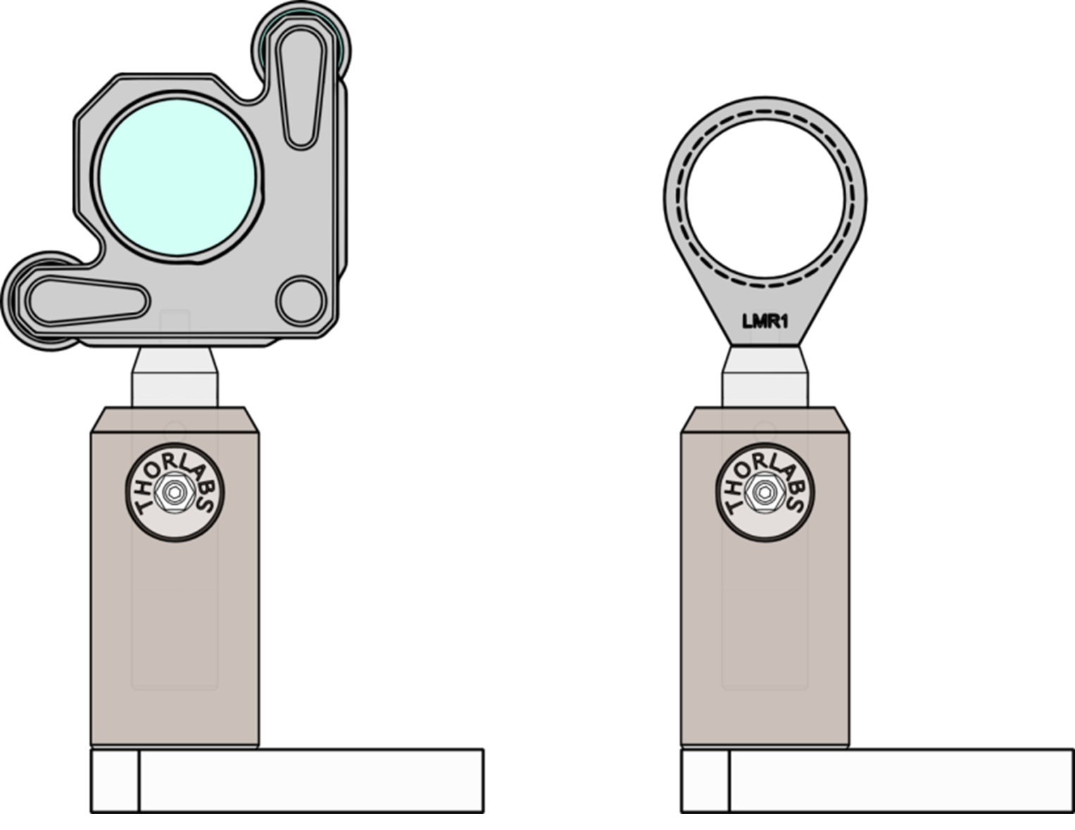
Pick a non-compound lens (not the fancy camera lenses) with focal length in the range 100-200 mm and assemble it in a lens mount with a retaining ring (see Figure 1). Recall that it’s very important that you do not handle optical components (lenses, mirrors, polarizers, wave plates, beam splitters, etc.) with your bare hands. The oils on your skin can damage the optics and degrade the light in your experiment. Always handle these components while using latex/nitrile gloves or finger cots.
Design and carry out an experiment to quantitatively answer the questions below. Consider carefully where to put the lens. Your data for this section can be used in the next section.
- Insert a lens (after the mirrors) into the beam path to change the divergence/convergence of the beam but keep its propagation direction the same.
- When this condition (the beam propagation direction is unchanged) is met, where does the beam intersect the lens? Note: This is the preferred method of adding a lens to an optical setup.
- Does the beam retain a Gaussian profile after the lens?
- What is the new beam waist \(w_0\) and where does it occur?
- What factors affect the beam profile after the lens?
- Does the measured \(w(z)\) match the Gaussian beam prediction? (Use the same fitting equation as before, with the new waist position \(z_w\) as a fit parameter.)
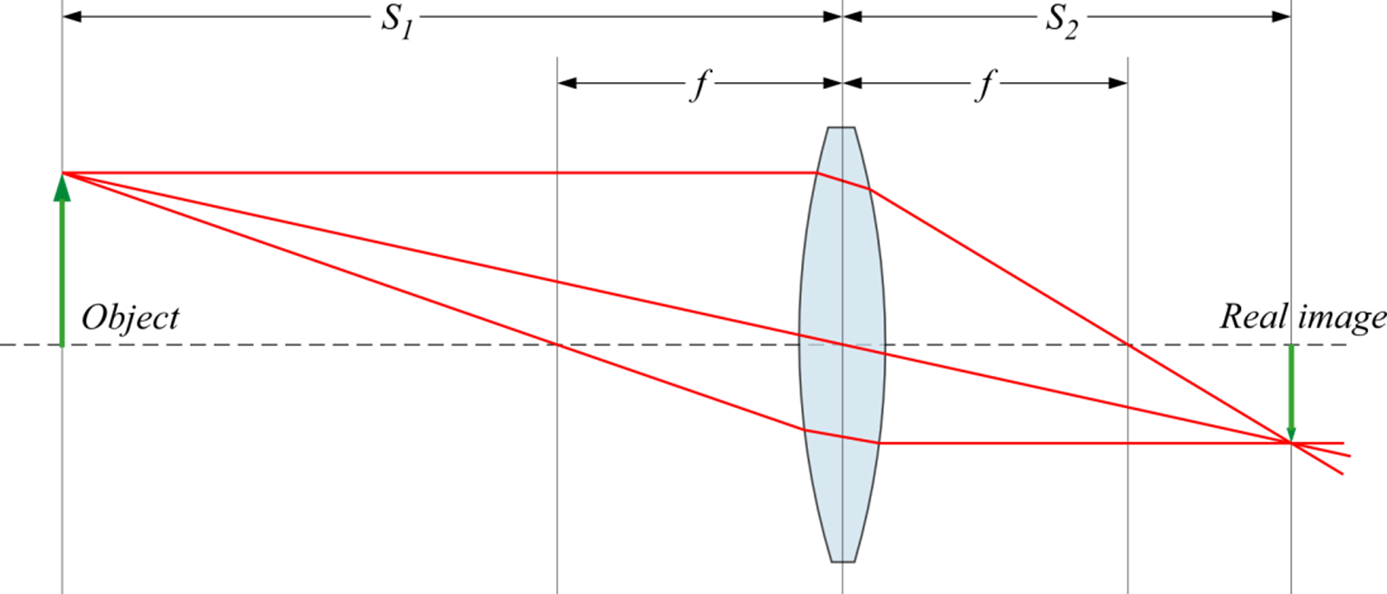
8.3 Quantitatively Modeling the Effect of a Lens
One of the simplest ways to model the effect of a lens is the thin lens equation, which is based on a ray model of light (see Figure 2).
\[ \frac{1}{S_1}+\frac{1}{S_2}=\frac{1}{f}\]
Redraw Figure 2 to show how it would change when the light is modeled as a Gaussian beam, rather than rays. In particular, where should the beam waists occur? What determines the relative size of the new beam waist \(w_0'\) compared to the original \(w_0\)?
Experimentally test the accuracy of the thin lens equation for the imaging of Gaussian beams. Follow this quantitative procedure:
Predict: Using the thin lens equation, calculate the predicted image position \(S_2\) from your measured object distance \(S_1\) and the lens focal length \(f\). Propagate the uncertainties in \(S_1\) and \(f\) to get an uncertainty in \(S_2\).
Measure: From your beam radius data, determine the actual position of the beam waist (image location) after the lens. Include uncertainty from your fit.
Compare: Calculate the discrepancy between predicted and measured image positions. Is the discrepancy smaller than the combined uncertainty? If \(|S_{2,predicted} - S_{2,measured}| < \sqrt{\sigma_{pred}^2 + \sigma_{meas}^2}\), the agreement is consistent with your uncertainties.
Interpret: If they disagree beyond uncertainties, this is not necessarily a mistake — the thin lens equation is a ray optics result that ignores diffraction. Proceed to question 3.
A better model: The thin lens equation assumes the beam waist acts like a point source, emitting spherical wavefronts. But a Gaussian beam’s wavefronts are flat at the waist and only gradually become spherical. The Rayleigh range \(z_R = \pi w_0^2/\lambda\) characterizes this transition. When the lens is many Rayleigh ranges from the waist (\(z_R \ll |S_1 - f|\)), the wavefronts at the lens are nearly spherical and the thin lens equation works. When \(z_R \gtrsim |S_1 - f|\), it doesn’t.
A modified thin-lens equation accounts for this (Self, “Focusing of spherical Gaussian beams,” Appl. Opt. 22, 658, 1983; see also Thorlabs: Modified Thin-Lens Equation for Laser Light for an accessible explanation):
\[ \frac{1}{S_1 + \dfrac{z_R^2}{S_1 - f}}+\frac{1}{S_2}=\frac{1}{f}\]
The conventional equation is recovered when \(z_R \ll |S_1 - f|\). Calculate the predicted \(S_2\) using this modified equation. Does it better agree with your measured value? The corresponding magnification is \(m = f / \sqrt{(S_1 - f)^2 + z_R^2}\).
Systematic errors: Under what conditions should the thin lens equation be most valid? Beyond the diffraction correction, what other effects could cause discrepancies? (Consider: thick lens effects, uncertainty in waist position, beam quality \(M^2 \neq 1\), lens aberrations.)
8.4 Peer Discussion: Comparing Results
If time permits, compare your thin lens test results with another group. This comparison helps identify systematic effects and builds confidence in your conclusions.
Compare measured image positions. Record each group’s values:
Group \(S_1\) (object distance) \(S_2\) (measured) \(S_2\) (predicted) Discrepancy Yours _______ _______ _______ _______ Other _______ _______ _______ _______ Investigate discrepancies: If results differ significantly, consider:
- Did you use different lenses or object distances?
- How did you each define “beam waist position”? (Peak intensity? Best fit location?)
- What systematic error sources might differ between setups?
Synthesize: What does the comparison tell you about the accuracy of the thin lens equation for Gaussian beams? If both groups found discrepancies in the same direction (e.g., both measured \(S_2\) shorter than predicted), what might that indicate about the model?
Document briefly in your notebook:
- Whether results agreed within uncertainties
- Key insight from the comparison
8.5 Advanced Investigation: Minimum Spot Size
If time permits, investigate the following:
- What determines the minimum spot size you can achieve with a lens?
- How does this relate to the concept of the “diffraction limit”?
- Try using a lens with shorter focal length. Does it produce a smaller spot? What are the tradeoffs?
9 Appendix: Troubleshooting Motor and DAQ Issues
This appendix provides troubleshooting guidance for common issues with motor control and data acquisition. These tips apply whether you’re using your own Week 3 code or the reference implementation.
9.1 Motor Issues
9.1.1 “Device not found” Error
- Check USB connection
- Verify serial number matches the display on the KST101
- Make sure no other software (APT User, Kinesis) is using the motor
9.1.2 Motor Doesn’t Move
- Ensure power is connected to the KST101
- Check that the stage isn’t at a travel limit
- Verify the stage type is configured correctly in Kinesis (ZST225B)
9.2 DAQ Issues
9.2.1 Voltage Reads Zero
- Check photodetector power
- Verify BNC cable connections to DAQ
- Make sure the beam actually hits the photodetector
9.2.2 Noisy Data
- Increase wait time between steps to let vibrations settle
- Check for mechanical vibrations in your setup
- Shield the photodetector from ambient light
- Average multiple DAQ readings per point
9.3 Reference Script Details
If you are using the reference implementation
(04_beam_profiler.py), here is its structure:
class BeamProfiler:
    def __init__(self, serial_number, daq_device="Dev1", daq_channel="ai0"):
        """Initialize with motor serial number and DAQ settings."""

    def connect(self):
        """Connect to motor controller, configure velocity."""

    def get_position(self):
        """Read current position in mm."""

    def move_to(self, position_mm):
        """Move to absolute position."""

    def read_voltage(self):
        """Read single voltage from DAQ."""

    def run_scan(self, step_size_mm, wait_time_ms, direction, max_steps):
        """Execute the automated scan with real-time plotting."""
The core measurement loop is the same as what you wrote in Week 3: move to position, wait for settling, read voltage, record data, repeat.
10 Deliverables and Assessment
Your lab notebook should include the following for this week:
10.1 Setup Validation
- Gain setting validation:
- Completed dark/signal measurement table
- Calculated SNR compared to Week 2 prediction
- Decision on whether gain setting needed adjustment
- Gain setting confirmation: your selected gain (_______ dB)
10.2 Beam Profile Without Lenses
- Automated vs. manual comparison: beam radius from both methods with uncertainties
- Multiple position measurements: table of \(z\) positions and corresponding \(w\) values
- Gaussian beam fit:
- Plot of \(w(z)\) data with fit curve
- Extracted \(w_0\) and \(z_w\) with uncertainties
- Comparison to theoretical prediction
10.3 Lens Investigation
- Experimental design: description of your measurement strategy
- Data and analysis:
- Beam profiles before and after lens
- New beam waist \(w_0\) and position \(z_w\)
- Test of whether beam remains Gaussian
- Thin lens equation test:
- Measured vs. predicted image position with uncertainties
- Whether the modified thin-lens equation resolves any discrepancy
- Peer comparison (if completed): other group’s results, whether results agreed, and key insight from discussion
10.4 Key Results Summary
| Measurement | Value | Uncertainty | Notes |
|---|---|---|---|
| \(w_0\) (no lens) | _______ | _______ | _______ |
| \(z_w\) (no lens) | _______ | _______ | _______ |
| \(w_0\) (with lens) | _______ | _______ | _______ |
| \(z_w\) (with lens) | _______ | _______ | _______ |
10.5 Reflection Questions
Your measured beam waist occurs 5 cm from the position predicted by the thin lens equation. List three possible explanations (including the possibility that the thin lens equation itself is approximate for Gaussian beams) and describe measurements that would distinguish between them.
You have 30 minutes remaining and want to improve your measurement of \(w_0\). You could either: (a) take more beam profiles at closely spaced \(z\) positions, or (b) take fewer profiles but with more averaging per profile. Which would you choose to minimize uncertainty in \(w_0\)? Justify your answer.
Predict-measure-compare reflection: Compare your Week 2 SNR predictions to your Week 4 measurements. What did you learn from this process? What would you do differently if characterizing a new instrument in the future?