PHYS 4430
Physics Undergraduate Labs
Michelson Interferometer & Precision Wavelength Measurement
Week 1
1 Where We Are in the Sequence
Week 1 of 2: Building and Understanding a Michelson Interferometer
This week you build a Michelson interferometer from scratch, develop a theoretical model for its behavior, and systematically explore how real-world imperfections affect its performance. The physical intuition and alignment skills you develop this week are essential for Week 2, where you’ll use the interferometer for precision wavelength measurement by fringe counting.
This week: Build interferometer → Develop theoretical model → Explore non-ideal behavior → Estimate position resolution
Next week: Add motorized stage → Count fringes during mirror motion → Measure laser wavelength
2 Learning Goals
After completing this week’s lab, you will be able to:
- Build and align a Michelson interferometer using standard optomechanical hardware.
- Construct the simplest idealized model of the Michelson (50/50 transmission/reflection, same polarization, perfect alignment) and use it to predict how the power on the photodetector depends on mirror position.
- Refine the ideal model to account for non-ideal features including imperfect beamsplitter ratios, polarization effects, and angular misalignment.
- Visually observe and explain how different kinds of misalignment produce different interference patterns.
- Apply the model and experimentally determined device parameters to estimate the smallest observable displacement change of one mirror.
3 Overview of Your Work
This week has three phases:
Prelab (~30 min, before lab). Derive how the power on the photodetector depends on the position of the moveable mirror. Predict what different misalignment patterns will look like. These predictions will be your reference point for everything that follows.
1. Build and align. You’ll set up the interferometer, align the beams, and observe interference fringes. You’ll compare your measured signal to your prelab prediction and observe the misalignment patterns you predicted.
2. Characterize non-ideal behavior. Real beamsplitters aren’t perfectly 50/50, and real beams don’t have identical polarizations. You’ll measure these imperfections, update your model, and use the refined model to estimate the position resolution of your interferometer.
See the detailed deliverables checklist at the end of this guide.
3.1 Connecting to Gaussian Beams
In Gaussian Beams, you learned to characterize measurement uncertainty through repeated sampling, noise characterization, and error propagation. Those skills apply here, but the dominant uncertainty sources are different. In the Michelson interferometer, key uncertainties come from the discrete nature of fringe counting, systematic biases in your acquisition, and the fidelity of your interferometer model — not just voltage noise. The reasoning framework (quantify uncertainty, compare to predictions, use uncertainty to make decisions) is the same; the specific sources you’ll investigate are new.
4 Prelab
Complete this prelab before your lab session (~30 min). You will compare these predictions to observations in lab. Before starting, read through the Deliverables and Assessment section at the end of this guide so you know what is expected for the week.
4.1 Ideal interferometer model
An ideal Michelson Interferometer splits the laser into two equally intense portions with the beam splitter. The ideal model should also keep the beam perfectly collimated and have a uniform polarization.
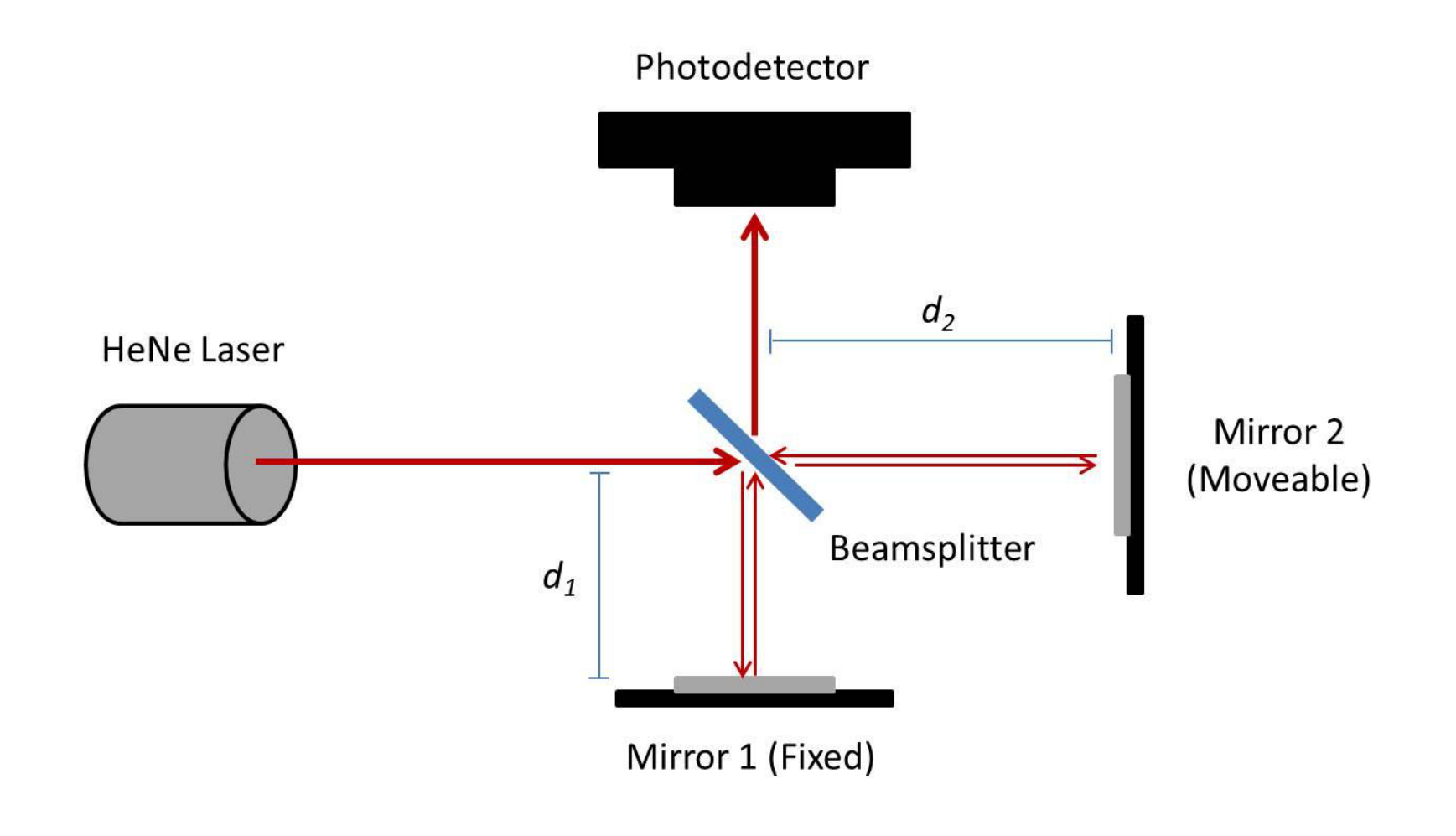
Assuming an idealized interferometer as shown in Figure 1 with a 50/50 beam splitter, single polarization of light, single wavelength, and perfect alignment, predict the power incident on the photodetector \(P\) as a function of mirror position \(d_2\). Model the electric field of the light as plane waves of the form \(\vec{E}_i(z,t) = \hat{n}\, E_i e^{i(kz - \omega t)}\), where \(\hat{n}\) is a unit vector along the polarization direction and \(k = 2\pi/\lambda\) is the wavenumber.
- Write your prediction \(P(d_2)\) as a mathematical expression and sketch the function.
- Explain how the four idealizations listed above are used in deriving \(P(d_2)\).
- How does the max and min power predicted by the function \(P(d_2)\) compare to the power incident upon the beamsplitter?
4.2 Misalignment pattern predictions
Qualitatively predict and sketch what the visible interference pattern between the two recombined beams will look like for the following cases. For each case, also sketch how the beam paths would differ from the ideal case to create this alignment condition.
- Two Gaussian beams of equal size are perfectly overlapped, but incident at different angles.
- Two Gaussian beams of different size are perfectly overlapped and incident at the same angle.
- Two Gaussian beams of equal size and incident at the same angle, but are only partially overlapped.
- Briefly explain each of your sketches.
5 Build and Align a Michelson Interferometer
5.1 Setting up the interferometer
Set up a Michelson Interferometer using a HeNe laser as shown in Figure 1. You’ll need:
- HeNe laser
- Non-polarizing beamsplitter
- Two adjustable mirrors
- Translation stage with manual micrometer (for Mirror 2)
- Photodetector
- Posts, post holders, and mounts
Mount Mirror 2 on the translation stage so that the micrometer controls its position along the beam axis. The micrometer lets you make fine, controlled adjustments to the path length \(d_2\) for this week’s measurements. In Week 2, you will swap the manual micrometer for a motorized actuator — the rest of the setup will remain intact.
5.2 Aligning the interferometer
Carefully align the interferometer by an iterative process of overlapping the beams. This requires two tiltable mirrors prior to the beam splitter, one to overlap the beams at a point close to the beamsplitter, and the other to overlap the beams at a point far from the beam splitter.
Predict, then observe: Why do you need 2 mirrors with 4 total knobs to get the beams overlapped? Why is one mirror not sufficient? (The misalignment analysis below will help you think through this in more detail.)
Once the beam is in good alignment at both points, look in a far plane for visible interference fringes. The better the alignment the wider the fringe spacing will be. You can use this to further refine the alignment of your apparatus.
Compare to your model: How does the measured power vs position \(P(d_2)\) compare to your prediction for the ideal case?
Save this as a script (e.g., voltage_monitor.py) and run it from the terminal. It opens a live plot window that updates as you adjust the micrometer. Close the window or press Ctrl+C to stop.
import nidaqmx
import numpy as np
import matplotlib.pyplot as plt
import time

fig, ax = plt.subplots(figsize=(8, 3))
line, = ax.plot([], [])
ax.set_xlabel("Time (s)")
ax.set_ylabel("Voltage (V)")
plt.ion()  # Turn on interactive mode for live updates
plt.show()

times, voltages = [], []
t0 = time.time()

with nidaqmx.Task() as task:
    task.ai_channels.add_ai_voltage_chan("Dev1/ai0")
    try:
        while True:
            times.append(time.time() - t0)
            voltages.append(task.read())

            # Keep the most recent 200 points
            times, voltages = times[-200:], voltages[-200:]

            line.set_data(times, voltages)
            ax.set_xlim(times[0], times[-1] + 0.1)
            ax.set_ylim(min(voltages) - 0.05, max(voltages) + 0.05)
            fig.canvas.flush_events()
            fig.canvas.draw_idle()

            time.sleep(0.1)  # ~10 readings/sec
    except KeyboardInterrupt:
        print("Stopped")

plt.close(fig)
This is optional—you can also use the oscilloscope for alignment.
5.3 Exploring misalignment patterns
Align your interferometer to observe each of the following patterns. Compare your observations to the predictions you made in the prelab and record what you actually see.
- Two Gaussian beams of equal size are perfectly overlapped, but incident at different angles.
- Two Gaussian beams of different size are perfectly overlapped and incident at the same angle.
- Two Gaussian beams of equal size and incident at the same angle, but are only partially overlapped.
- How do your observations compare to your prelab predictions? Note any differences and explain them.
6 Measurable Properties of the Michelson
The following steps will guide you through refining your idealized model to develop a more realistic model of the Michelson interferometer that you built.
6.1 Effect of angular misalignment
Without a perfect alignment, fringes will always be observable at large distances from the beam splitter. A small \(\delta\theta\) between the two incident beams can cause deviation from a good alignment.
Predict and sketch: How will a small \(\delta\theta\) affect \(P(d_2)\), the power incident on the photodetector as a function of mirror position?
6.2 Non-ideal beamsplitter
In the most simple model of the Michelson interferometer, we assumed power was distributed 50/50 from the beamsplitter.
- What is the actual power ratio between the two arms of your interferometer? What are the electric field reflection and transmission coefficients for the beam splitter?
- Use the coefficients to predict the power on the photodetector as a function of mirror position \(P(d_2)\). Compare your prediction to the ideal case and to measurements. Is the discrepancy between your predicted and measured \(P_{max}\) and \(P_{min}\) within the uncertainty you would expect from your photodetector noise floor?
6.3 Polarization effects
Another assumption of the simple model was that the electric fields in each arm had identical polarization when the beams recombine.
- Should the beamsplitter in the Michelson be a polarizing beamsplitter or a non-polarizing beamsplitter? Why?
- Does the measured signal \(P(d_2)\) depend on the incident polarization of the light? Is there a preferred polarization for the incident light on the beam splitter?
- If you rotate the polarization of one arm of the interferometer by \(\pi/2\) before it recombines at the beamsplitter, how will the power on the photodetector \(P(d_2)\) change from the idealized case? (If a quarter-wave plate, a.k.a \(\lambda/4\) plate, is available, use it to change the polarization in one arm of the interferometer and test your answer.)
6.4 Position resolution
One extremely common application of an interferometer is for sensitive measurement of displacement because very small displacements (sub-wavelength) cause large changes in the power measured on the photodetector.
Use what you have learned about your particular Michelson interferometer to estimate the position resolution of your interferometer. This requires you to estimate \(d(d_2)/dP\) and determine an estimate for the smallest observable change in power \(\delta P_\text{min}\). To estimate \(\delta P_\text{min}\), consider what limits the smallest detectable change in photodetector voltage — you characterized this in Gaussian Beams Week 2 when you measured the DAQ noise floor. If you did not complete that lab, take repeated readings of the photodetector output at a fixed mirror position and use the standard deviation as your noise estimate. Explain all your reasoning.
7 Deliverables and Assessment
Your lab notebook should include the following for this week. This checklist represents minimum expectations — your notebook should also include any unexpected observations, failed approaches that informed your understanding, and questions that arose during the lab.
7.1 Prelab (complete before lab, ~30 min)
- Ideal model derivation: \(P(d_2)\) expression with sketch and explanation of the four idealizations
- Misalignment pattern predictions: sketches for all four cases (a-d) with beam path diagrams and explanations
7.2 In-Lab Documentation (recorded during lab)
- Optical setup diagram showing laser, beamsplitter, mirrors, and photodetector positions
- Ideal model comparison: comparison of measured \(P(d_2)\) to your prelab prediction for the ideal case
- Alignment observations: description of fringe patterns during alignment
- Misalignment pattern observations: observed patterns for cases (a-d), comparison to prelab predictions
- Angular misalignment prediction: sketch of how \(\delta\theta\) affects \(P(d_2)\)
- Beamsplitter characterization: measured power ratio, calculated field coefficients, refined \(P(d_2)\) prediction
- Polarization observations: answers to all three polarization questions with measurements
7.3 Analysis (can be completed after lab)
- Position resolution estimate: complete derivation of \(d(d_2)/dP\), estimate of \(\delta P_\text{min}\), and final position resolution with reasoning
- Model comparison: quantitative comparison of ideal vs. refined model vs. measurements
7.4 Preparation for Week 2
- Complete the Week 2 prelab (~30-45 min): The prelab walks you through deriving the fringe counting formula, calculating expected fringe counts, and a synthetic fringe counting exercise. This is your primary preparation for next week.
- Review the DAQ and motor control guides: Review the NI-DAQmx streaming acquisition section and the Thorlabs Motors velocity control section. You used these tools in Gaussian Beams; the new patterns for this lab (continuous DAQ streaming and constant-velocity motion) are described in the Week 2 guide.